↗ OpenReview ↗ NeurIPS Homepage ↗ Chat
TL;DR#
Many real-world systems are modeled as networks of interacting entities where uncovering the hidden structures is vital. Traditional methods often struggle with irregularly sampled data and incomplete observations, which limit the accuracy and reliability of structural inference. These limitations significantly hinder our understanding and predictive capabilities for various domains, including physics, biology, and social sciences.
To tackle these challenges, the authors propose SICSM, a novel framework that combines the robust temporal modeling of selective State Space Models (SSMs) with the flexible structural inference of Generative Flow Networks (GFNs). This approach effectively learns input-dependent transition functions to handle irregular sampling intervals and approximates the posterior distribution of the system’s structure by aggregating dynamics across temporal dependencies. The results show that SICSM significantly outperforms existing methods, particularly when dealing with incomplete and irregularly sampled data, showcasing its potential as a valuable tool for scientific discovery and systems analysis across various disciplines.
Key Takeaways#
Why does it matter?#
This paper is crucial for researchers working with complex dynamical systems, especially those with irregularly sampled data or incomplete observations. It provides a robust and accurate method for structural inference, pushing the boundaries of what’s possible in network reconstruction. The proposed approach paves the way for improved system diagnostics, scientific discovery, and predictive modeling in diverse fields.
Visual Insights#

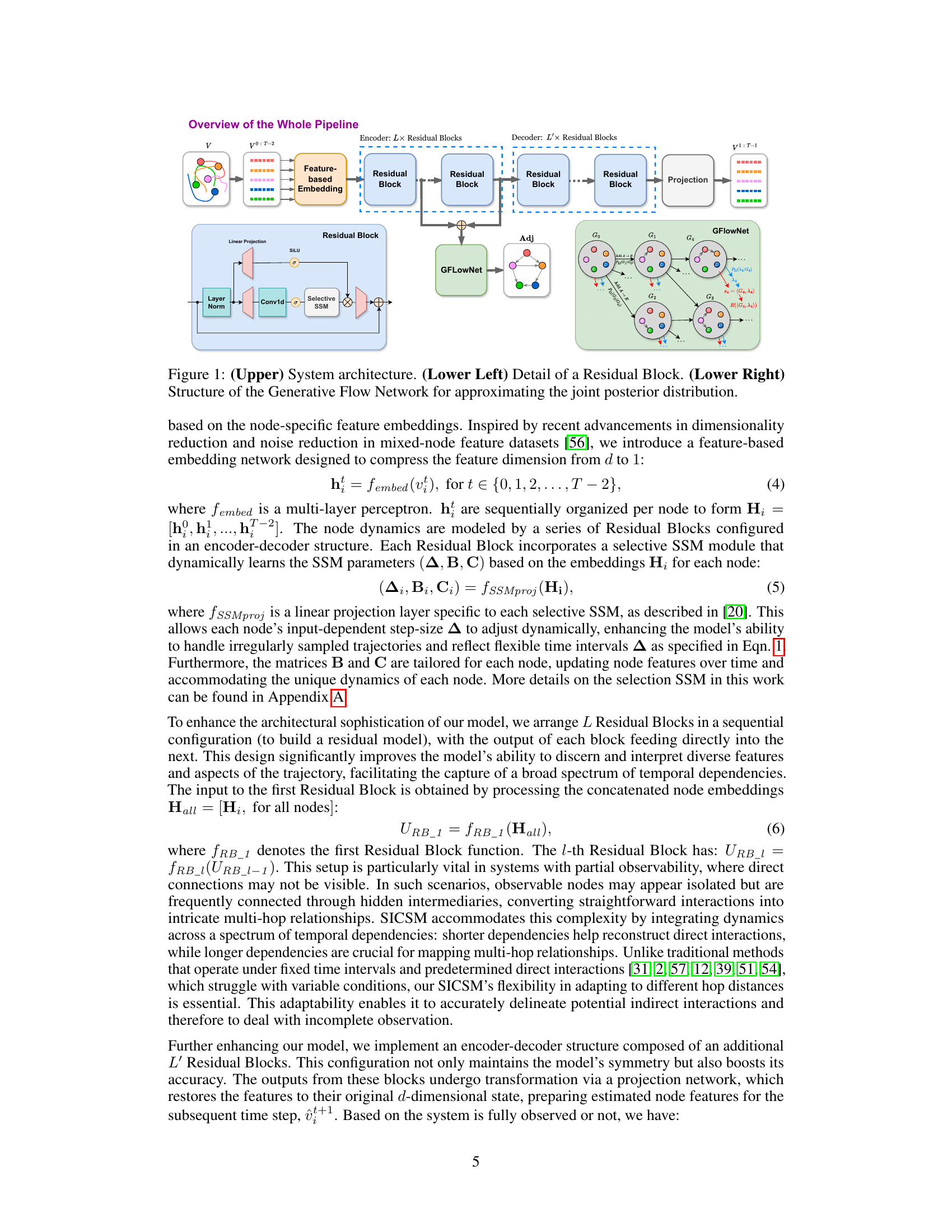
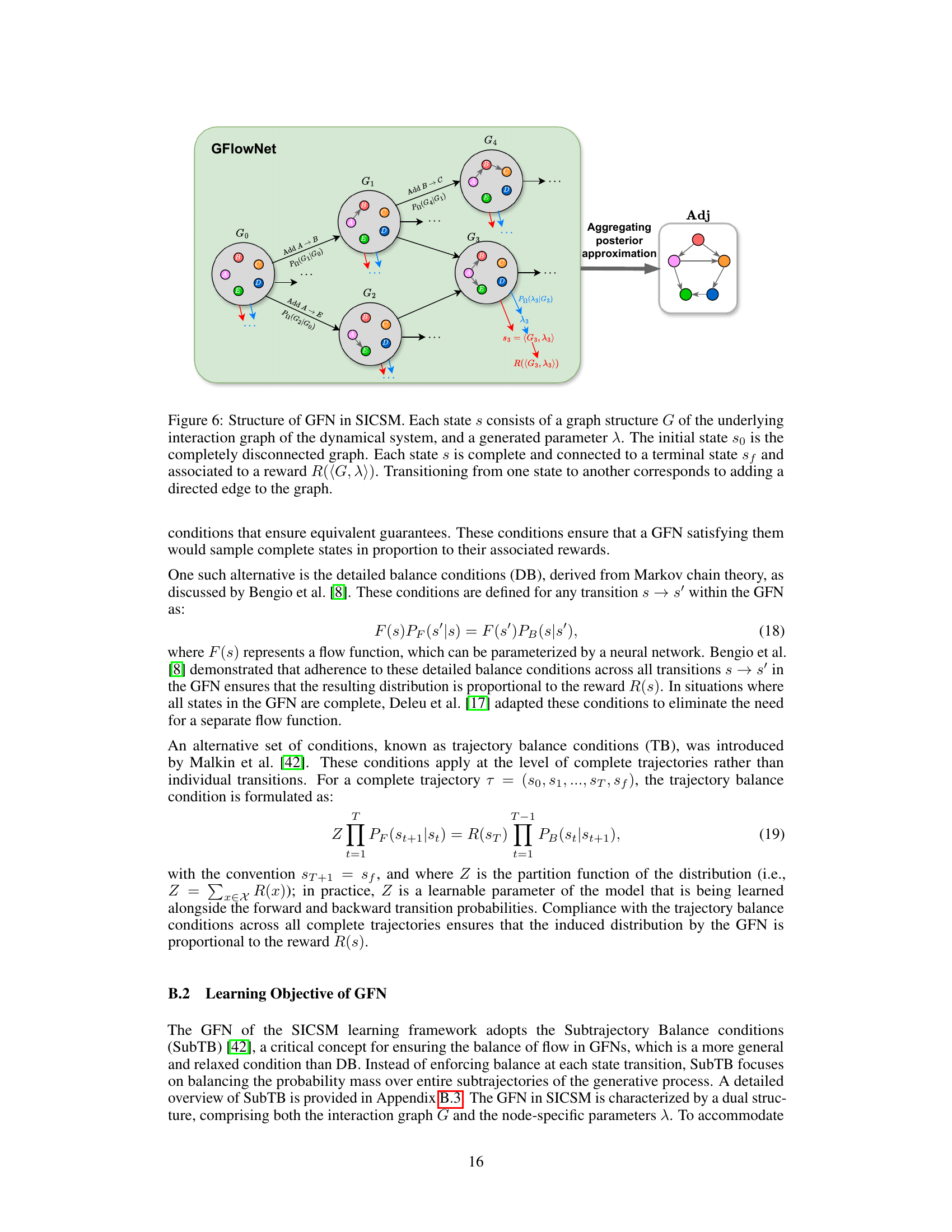
This figure provides a comprehensive overview of the proposed SICSM framework. The upper part illustrates the overall system architecture, outlining the flow of data through feature embedding, residual blocks with selective SSMs, and generative flow networks (GFNs). The lower left section zooms into a single residual block, showcasing the internal components and data processing steps. The lower right section focuses on the GFN, detailing how it approximates the joint posterior distribution of the system’s structure. This detailed visualization helps to understand the complex interplay of components within the SICSM model and its function in structural inference.

This table presents the results of an ablation study evaluating the impact of using different numbers of residual blocks in the SICSM model on the counts of multi-hop negative edges (incorrectly predicted edges spanning more than one hop) and true positive edges (correctly predicted edges). The experiment used the VN_SP_15 dataset with only 12 out of 15 nodes sampled, and the results are averaged over 10 independent runs. The table shows how combining outputs from multiple residual blocks (e.g., using 1-7 blocks) gradually improves the accuracy of edge prediction, reducing the number of false negative predictions (missing edges) and increasing the number of true positives. The results highlight the importance of aggregating dynamic information from multiple layers in SICSM for better structural inference in partially observed systems.
In-depth insights#
Irregular Data Handling#
Handling irregular data is crucial for accurate modeling of real-world dynamical systems. Irregular sampling intervals introduce complexities in learning temporal dependencies, as traditional methods often assume uniform time steps. The paper addresses this by using Selective State Space Models (SSMs), which adapt to non-uniform time intervals by learning input-dependent transition functions. This enhances the model’s accuracy in approximating the posterior distribution of the system’s structure. By aggregating dynamics across diverse temporal dependencies and channeling them into a Generative Flow Network (GFN), the system adeptly handles the challenges posed by irregularly sampled trajectories. This approach ensures robust temporal modeling and precise inference, even in scenarios with complex interactions and partially observed systems. The results demonstrate that this method significantly outperforms existing methods, particularly when dealing with irregular sampling.
GFN for Inference#
Utilizing Generative Flow Networks (GFNs) for structural inference presents a powerful approach to address challenges inherent in modeling complex dynamical systems. GFNs excel at capturing complex, high-dimensional probability distributions, making them well-suited for approximating the posterior distribution of a system’s structure, particularly when dealing with partially observed data or irregular sampling. The GFN’s ability to sample from this distribution enables efficient exploration of the vast space of possible structures, enabling the identification of the most probable network configuration. By integrating GFNs with temporal modeling techniques like Selective State Space Models (SSMs), a robust framework emerges, one that seamlessly handles the challenges of both irregular sampling intervals and incompletely observed nodes. The combination leverages the strengths of both approaches: SSMs providing robust temporal modeling and GFNs the flexible structural inference.
Adaptive SSMs#
Adaptive State Space Models (SSMs) represent a significant advancement in modeling dynamic systems, particularly those exhibiting non-stationary behavior. Their key strength lies in the ability to adjust model parameters in response to changing data characteristics, unlike traditional SSMs which assume fixed parameters. This adaptability is crucial for accurate representation of systems whose dynamics evolve over time, influenced by internal state changes or external factors. Adaptive methods incorporate mechanisms like online learning or parameter tuning based on incoming data, enabling the model to continuously adapt to new information. This allows for more robust predictions and a more precise understanding of the system’s underlying processes. Implementation strategies vary, with some using recurrent neural networks to dynamically adjust transition matrices, while others leverage reinforcement learning or Bayesian methods for online parameter estimation. A major challenge in adaptive SSMs is finding the optimal balance between adapting quickly enough to capture changing dynamics and avoiding overfitting to noise or short-term fluctuations. Therefore, careful consideration of hyperparameters is essential, often involving techniques such as regularization, early stopping, or adaptive learning rates. Overall, adaptive SSMs show great promise for enhancing the accuracy and robustness of dynamic system modeling across various domains.
Partial Obs. Robustness#
The robustness of a system to partial observation is a crucial aspect to consider when evaluating its performance in real-world scenarios. A system’s ability to accurately infer structure and predict behavior even with missing or incomplete data is a key indicator of its reliability. This robustness is particularly important for complex dynamical systems, where the underlying structure can be challenging to uncover from limited observations. In the context of the described structural inference framework, partial observation robustness is demonstrated by the model’s consistent performance across different levels of data completeness. This involves both regularly and irregularly sampled trajectories, and highlights the model’s ability to handle non-uniform data availability, a common limitation in various disciplines. The robustness is evaluated through rigorous experimentation using diverse datasets, with a focus on scenarios where only a fraction of system nodes are observed. The evaluation metric, area under the receiver operating characteristic curve (AUROC), provides a quantitative assessment of the model’s structural inference accuracy, confirming its resilience even when faced with significant data limitations. The consistently high AUROC scores highlight the effective integration of adaptive learning mechanisms and model architecture for handling missing information.
Future Research#
Future research directions stemming from this work on structural inference of dynamical systems using Conjoined State Space Models (SICSM) should prioritize extending SICSM’s capabilities to handle dynamic graphs, where the underlying network structure itself evolves over time. This requires developing methods that can adapt the model’s parameters and structure as new connections emerge and existing ones change or disappear. A second crucial area is improving computational efficiency. While SICSM offers promising results, its current implementation, especially the GFN and selective SSM modules, is computationally expensive. Investigating algorithmic optimizations or hardware acceleration techniques is crucial to make SICSM more practical for real-world applications involving larger datasets and more complex systems. A third avenue for future research is to explore handling incomplete or noisy data with more sophisticated methods. The current SICSM approach utilizes a selective mechanism but further development could explore other approaches such as using imputation strategies, advanced noise-reduction techniques, and data augmentation. Finally, rigorous evaluation on diverse real-world datasets is vital to truly understand SICSM’s robustness and generalizability. The current study relies primarily on synthetic datasets, leaving open questions regarding performance in real-world settings characterized by messy, complex data.
More visual insights#
More on figures

The figure shows the AUROC values for different methods under varying degrees of irregular sampling. It compares the performance of SICSM against other state-of-the-art methods by showing how their AUROC changes as the number of time steps in the irregularly sampled data decreases. The consistency of SICSM’s performance across different levels of irregularity is highlighted.

This figure displays the Area Under the Receiver Operating Characteristic (AUROC) curve for several structural inference methods. The x-axis represents the number of irregularly sampled time steps, ranging from 10 to 49, while the y-axis shows the AUROC, expressed as a percentage. Each subplot represents a different dataset, demonstrating the performance of various methods across different sampling rates. The aim is to showcase how the methods’ AUROC changes in the presence of irregular time series data.

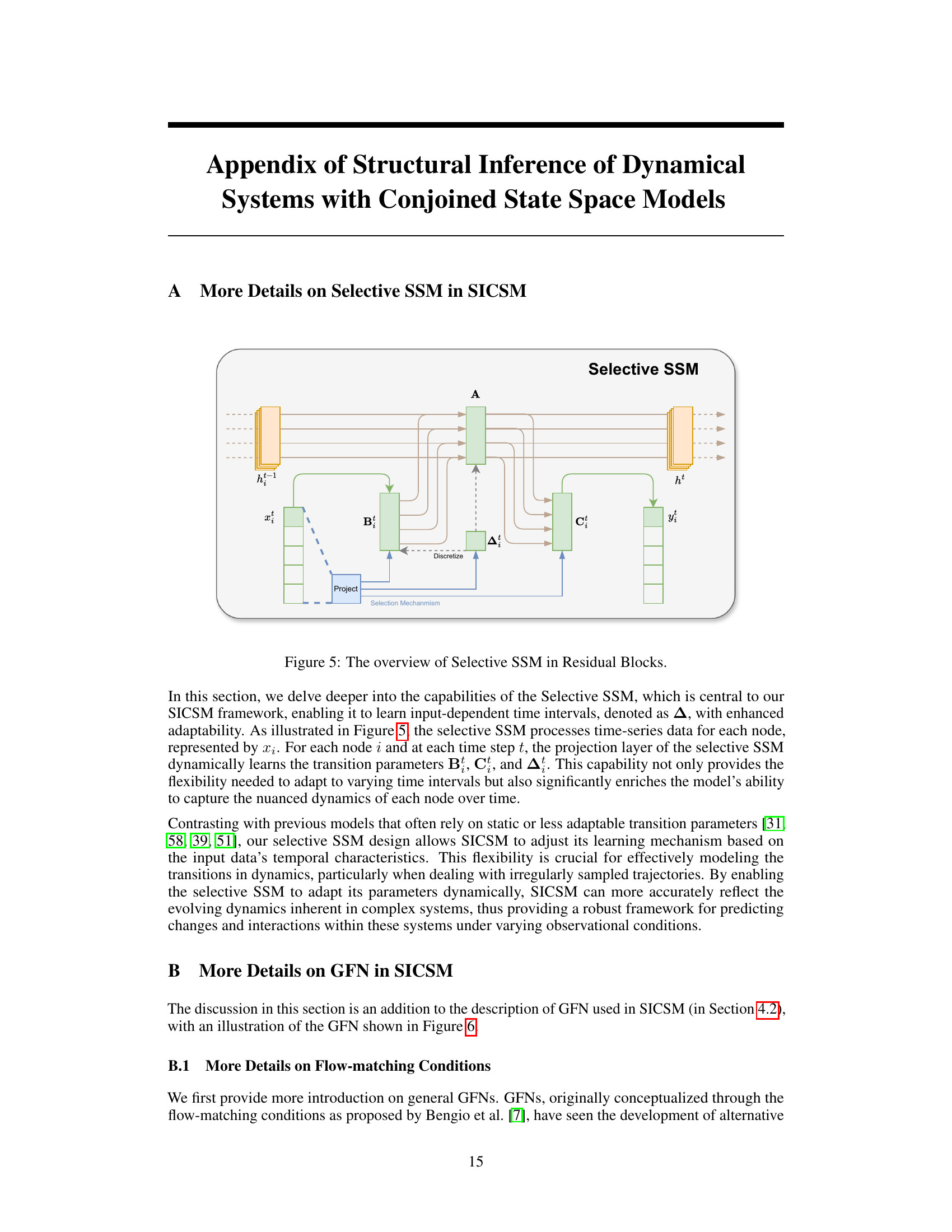
This figure shows the architecture of a Selective State Space Model (SSM) within a Residual Block. The input to the SSM includes the previous hidden state (ht-1) and the current input (xt). The input (xt) first goes through a projection layer (Bit) before being processed by the SSM. The SSM contains a dynamic state transition matrix (A) and an output projection layer (Cit). A selection mechanism determines which parts of the input sequence flow into the hidden states. The output of the SSM is the current hidden state (ht) and the current output (yit). The process incorporates a discretization step (Δt) to handle varying time intervals in the input data. The design is meant to adapt to irregularly sampled time series data, which is a key feature of the SICSM framework.
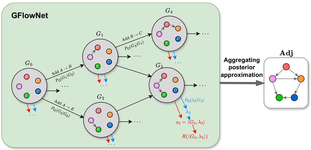
This figure provides a comprehensive overview of the SICSM pipeline. The upper part illustrates the overall architecture, showing the flow of data through the encoder (multiple Residual Blocks with selective SSMs), feature-based embedding, and generative flow network (GFN) for structure approximation. The lower left section zooms in on a single residual block, detailing the internal structure of the selective SSM module. Finally, the lower right section provides details about the GFN’s architecture, illustrating how it approximates the posterior distribution. The figure effectively visualizes how the different components of SICSM work together to achieve accurate structural inference.

This figure displays the AUROC (Area Under the Receiver Operating Characteristic curve) values for several structural inference methods across different numbers of irregularly sampled time steps, ranging from 10 to 49. Each subplot represents a different dataset. The results are averaged over 10 trials to show the average performance and consistency of each method under irregular sampling conditions. The consistent x and y axes facilitate easy comparison between the methods and across the various datasets.

This figure presents the Area Under the Receiver Operating Characteristic (AUROC) curves for several structural inference methods across various datasets. The x-axis represents the number of irregularly sampled time steps, ranging from 10 to 49, while the y-axis displays the AUROC values (in percentage). The plot shows how different methods perform under varying levels of data irregularity. Each subplot represents a different dataset, allowing for a comparison across various scenarios.

This figure displays the Area Under the Receiver Operating Characteristic curve (AUROC) for several structural inference methods across different numbers of irregularly sampled time steps. The AUROC score measures the accuracy of each method in predicting the structure of a dynamical system. The x-axis shows the number of time steps, and the y-axis shows the AUROC score (as a percentage). The results are averaged over ten trials, and error bars (standard deviations) are displayed. Each subplot represents a different dataset, showcasing the performance of the methods under different data conditions.

This figure displays the average AUROC scores achieved by SICSM and several baseline methods (NRI, MPM, ACD, iSIDG, RCSI, JSP-GFN) across four different datasets (VN_SP_50, VN_SP_100, VN_NS_50, VN_NS_100) under various levels of prior knowledge integration (0%, 10%, 20%, 30%). It illustrates how the performance of each method changes with the incorporation of prior knowledge. The results highlight the effectiveness of SICSM, showing consistent improvement across datasets and knowledge levels.
This figure illustrates the overall architecture of the proposed SICSM model, which combines selective state space models (SSMs) and generative flow networks (GFNs). The upper panel depicts the entire system, showing how the input trajectories are processed through multiple residual blocks (each containing a selective SSM) to aggregate dynamic features. These aggregated dynamics are then fed into a GFN for structure inference. The lower-left panel zooms in on a single residual block, showing its internal structure which includes a selective SSM to handle irregular sampling. Finally, the lower-right panel details the GFN structure used for approximating the posterior distribution of the system’s structure. Each of these components plays a crucial role in the model’s ability to accurately infer the structure from complex dynamics with non-uniform sampling.

This figure shows a comparison of the edge features computed using the exact posterior distribution against those approximated using the generative flow network (GFN) within the SICSM model. The x-axis represents the exact posterior values, while the y-axis represents the values estimated by SICSM’s GFN. The strong correlation (r = 0.9983) indicates that SICSM effectively approximates the edge feature probabilities from the exact posterior distribution. This demonstrates the accuracy of the GFN component of SICSM in learning and sampling from the complex posterior distribution over the graph structure.
More on tables

This table presents the statistics of three PEMS datasets, including the number of nodes, edges, time steps, and the missing ratio. The PEMS datasets are derived from the California Caltrans Performance Measurement System and consist of traffic flow data aggregated into 5-minute intervals. The adjacency matrix is constructed using a thresholded Gaussian kernel based on road network distances. The missing ratio indicates the percentage of missing data points in each dataset.

This table shows how the number of residual blocks in the encoder of the SICSM model scales with the number of nodes (n) in the graph. As the number of nodes increases, more residual blocks are used to capture the increasing complexity of the system’s dynamics. This reflects an adaptive design where the model’s architecture adjusts to handle the varying difficulty of the inference task, depending on the size of the system being modeled.

This table presents the performance evaluation of three methods (JSP-GFN, SIDEC, and SICSM) on three real-world datasets (PEMS03, PEMS04, and PEMS07). The AUROC (Area Under the Receiver Operating Characteristic curve) is a common metric for evaluating the accuracy of a model’s predictions. Higher AUROC values indicate better performance. The table shows that SICSM consistently outperforms the other two methods across all three datasets.

This table presents the results of an experiment evaluating the impact of using different numbers of residual blocks in the SICSM model on the accuracy of reconstructing the graph structure for a dataset with 12 nodes. The model’s performance is measured by the average counts of multi-hop negative edges (incorrectly identified connections) and true positive edges (correctly identified connections). Results are averaged over 10 runs for each configuration.

This table presents the AUROC (Area Under the Receiver Operating Characteristic curve) scores achieved by the proposed SICSM model using different neural networks (Transformer, LSTM, GRU) within its residual blocks. The experiment was performed under conditions of irregularly sampled time steps and partially observed nodes in the VN_SP_15 dataset. The AUROC is a common metric for evaluating the performance of binary classifiers in which a higher score (closer to 1.0) implies better performance.
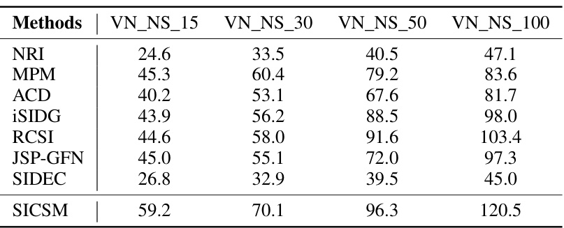
This table presents the training times, in hours, for various structural inference methods (NRI, MPM, ACD, iSIDG, RCSI, JSP-GFN, SIDEC, and SICSM) across four different datasets (VN_NS_15, VN_NS_30, VN_NS_50, VN_NS_100) with varying node counts. The results highlight the computational cost of each method and its scaling behavior with dataset size. SICSM demonstrates superior inference accuracy but at the cost of increased training time.

This table compares the performance of JSP-GFN and SICSM against the exact posterior distribution for small graphs (5 nodes). It evaluates both the accuracy of edge feature approximation and the cross-entropy between the sampling distribution of parameters λ and the true posterior distribution. The results show that both methods provide good approximations, with SICSM showing slightly better performance.
Full paper#
