↗ OpenReview ↗ NeurIPS Homepage ↗ Chat
TL;DR#
Fine-tuning pre-trained models is a common practice in AI, but it often suffers from a significant drop in accuracy when encountering classes not seen during fine-tuning. This phenomenon, often attributed to catastrophic forgetting, has been a major challenge for researchers. This paper challenges this conventional wisdom.
The researchers systematically investigated the problem and discovered that the drop in accuracy is not due to a loss or degradation of learned features regarding the unseen classes but rather a scaling issue (logit) between the seen and unseen classes. They demonstrate that a simple post-processing calibration method could effectively restore the model’s performance on the unseen classes. This significantly simplifies how we improve models and has broad implications for future research.
Key Takeaways#
Why does it matter?#
This paper is crucial because it addresses a critical issue in fine-tuning pre-trained models, a widely used technique in modern AI. By revealing that the problem isn’t feature loss but rather logit scale discrepancies, it opens exciting new avenues for research into calibration techniques and more efficient model adaptation. Its findings are broadly applicable and have the potential to significantly improve the performance and utility of fine-tuned models across various domains.
Visual Insights#
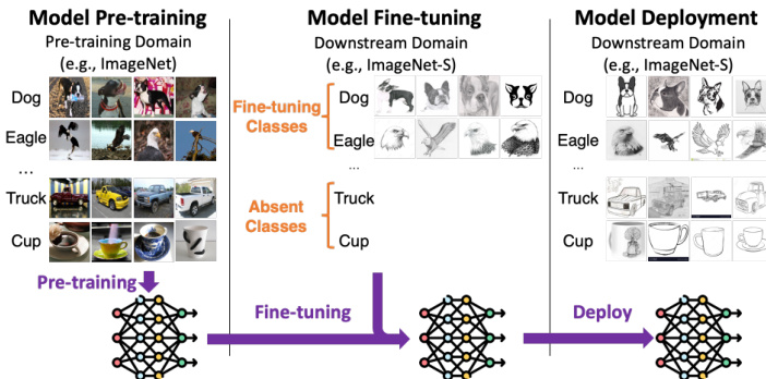
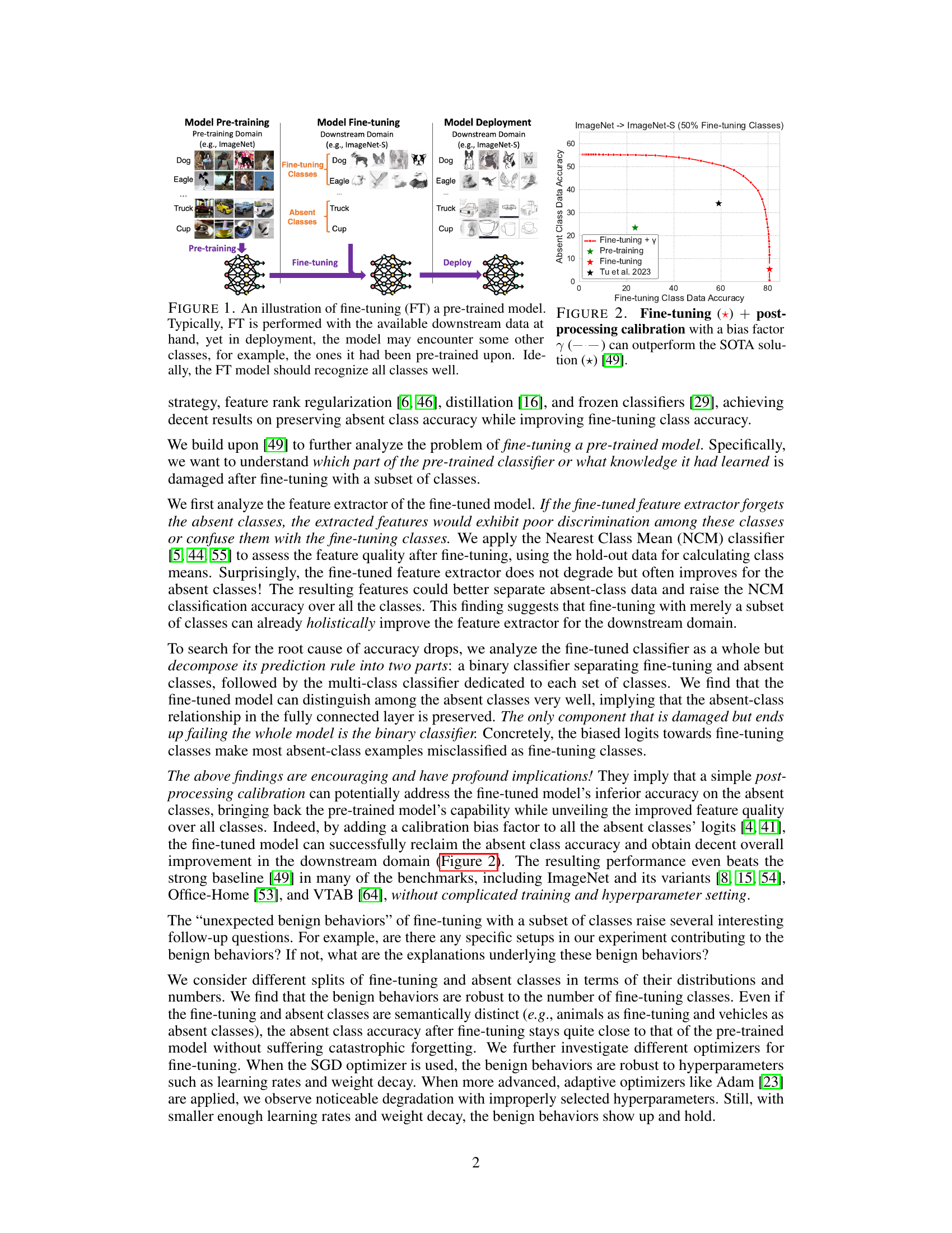
This figure illustrates the process of fine-tuning a pre-trained model. The left panel shows the pre-training phase using a dataset with multiple classes (dog, eagle, truck, cup). The middle panel depicts the fine-tuning phase, where the pre-trained model is further trained on a smaller subset of classes from the pre-training dataset (dog, eagle, truck). The right panel shows the deployment phase where the model is used on a dataset including both the classes it was fine-tuned on and classes that were in the pre-training data but not included in the fine-tuning phase (cup). Ideally, the fine-tuned model should be able to recognize all the classes from the pre-training dataset.

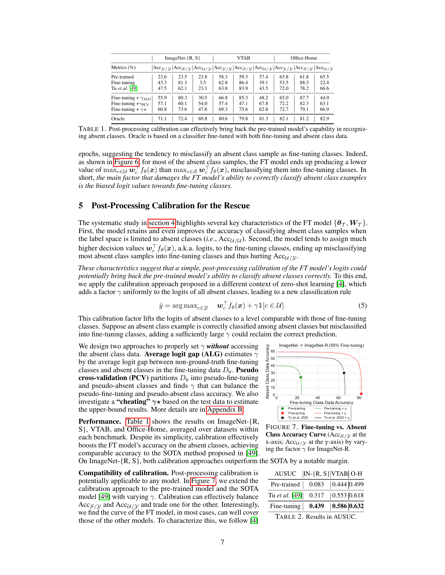
This table presents the performance comparison of different methods on three benchmark datasets (ImageNet-{R, S}, VTAB, and Office-Home). It compares the accuracy of pre-trained models, models fine-tuned on a subset of classes, a state-of-the-art (SOTA) fine-tuning method, and models with post-processing calibration. The metrics presented include overall accuracy (Accy), accuracy on fine-tuning classes (Accs/y), accuracy on absent classes (Accu/y). An oracle model, trained with both fine-tuning and absent classes, is included as an upper bound for comparison. The table demonstrates the effectiveness of post-processing calibration in recovering the accuracy of absent classes that was lost during the fine-tuning process.
In-depth insights#
Fine-tuning’s Perils#
Fine-tuning, while a powerful technique for adapting pre-trained models, presents significant challenges. Catastrophic forgetting, where the model loses previously learned knowledge, is a major concern, especially when fine-tuning on a limited subset of classes. This can lead to a substantial drop in performance on unseen classes, rendering the model less versatile and less useful for broader applications. Calibration issues frequently arise, where the model’s confidence scores are misaligned between fine-tuned and original classes, impacting accuracy and reliability. Overfitting to the fine-tuning data is another risk, compromising the model’s ability to generalize to new, unseen data. Addressing these perils requires careful consideration of techniques like regularization, data augmentation, and post-processing calibration, but a complete solution remains elusive and is an active area of research. Understanding the underlying causes of these issues is critical to developing more robust and reliable fine-tuning methods.
Calibration’s Rescue#
The heading “Calibration’s Rescue” aptly encapsulates a core finding: fine-tuning pre-trained models, while efficient for specific tasks, can negatively impact performance on unseen classes. This degradation isn’t due to forgotten knowledge or deteriorated feature extraction; instead, the issue stems from logit scale discrepancies between fine-tuned and original classes. The solution presented is surprisingly simple: post-processing calibration. By adjusting logit scales, the model recovers its ability to classify unseen data, even revealing improved feature discrimination in those areas. This highlights that the problem isn’t inherent to fine-tuning itself but to a calibration issue that can be easily addressed, a critical insight for future model development and deployment.
Feature Analysis#
A thorough feature analysis within a research paper would involve a multi-faceted investigation. It would start with a clear definition of what constitutes a “feature” in the context of the study. Then, the analysis should delve into the methods used for feature extraction and selection. This could include dimensionality reduction techniques, feature engineering strategies, and algorithms for selecting a relevant subset of features. Crucially, the analysis needs to address the quality of the extracted features, perhaps using quantitative metrics to assess their discriminative power and relevance. Visualizations like t-SNE plots could aid in understanding feature relationships and clustering. Furthermore, a rigorous feature analysis should explore how features change over time or across different experimental conditions. This dynamic perspective is vital for understanding the impact of interventions or treatments. Finally, the analysis should connect features back to the paper’s overarching goals. How do the chosen features relate to the conclusions and interpretations presented? A strong feature analysis is essential for providing a solid foundation and justifying the results of the study.
Optimizer Effects#
An in-depth exploration of optimizer effects in the context of fine-tuning pre-trained models reveals crucial insights into model behavior and performance. Different optimizers exhibit varying sensitivities to hyperparameter settings, impacting the model’s ability to generalize and retain knowledge from pre-training. While SGD demonstrates robustness across diverse hyperparameters, adaptive optimizers like Adam require careful tuning to avoid performance degradation. Understanding optimizer sensitivity is critical for achieving optimal fine-tuning results and underscores the need for careful selection and configuration of the optimization algorithm. The choice of optimizer can significantly impact both the fine-tuning classes’ and absent classes’ accuracies, highlighting the importance of this parameter in managing catastrophic forgetting and improving overall model performance. Further research could explore the interplay between optimizer choice, pre-training strategies, and downstream task characteristics to gain a more comprehensive understanding of fine-tuning optimization.
Future Work#
Future research could explore several promising avenues. Extending the calibration techniques beyond simple bias adjustments to achieve more robust performance across diverse datasets is crucial. Investigating the theoretical underpinnings of the observed benign behaviors of fine-tuning, particularly the preservation of absent class relationships, warrants further investigation. Developing novel fine-tuning strategies that explicitly address the logit scale discrepancies without sacrificing the positive feature improvements observed could significantly enhance practical applications. Moreover, applying these insights to different fine-tuning methods (e.g., parameter-efficient methods) and various model architectures would broaden the applicability and impact. Finally, a comprehensive empirical study across a wider range of domains and tasks is needed to solidify the robustness and generality of these findings.
More visual insights#
More on figures
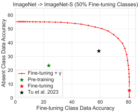
This figure shows the absent class data accuracy plotted against the fine-tuning class data accuracy. The black star represents the state-of-the-art (SOTA) result from a previous study (Tu et al. 2023). The red line shows the results of fine-tuning the model with a post-processing calibration applied, demonstrating that calibration significantly improves the absent class accuracy, surpassing the previous SOTA.

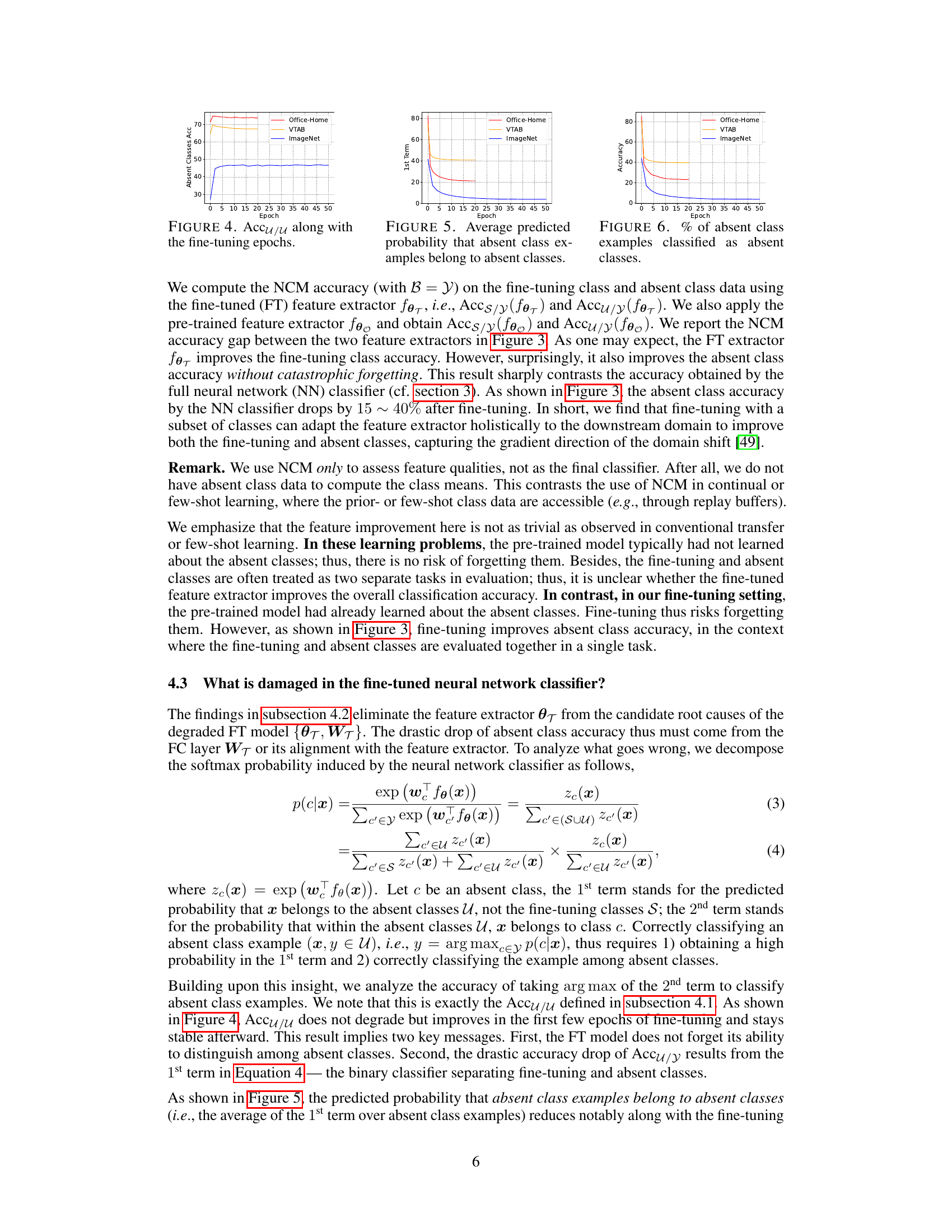
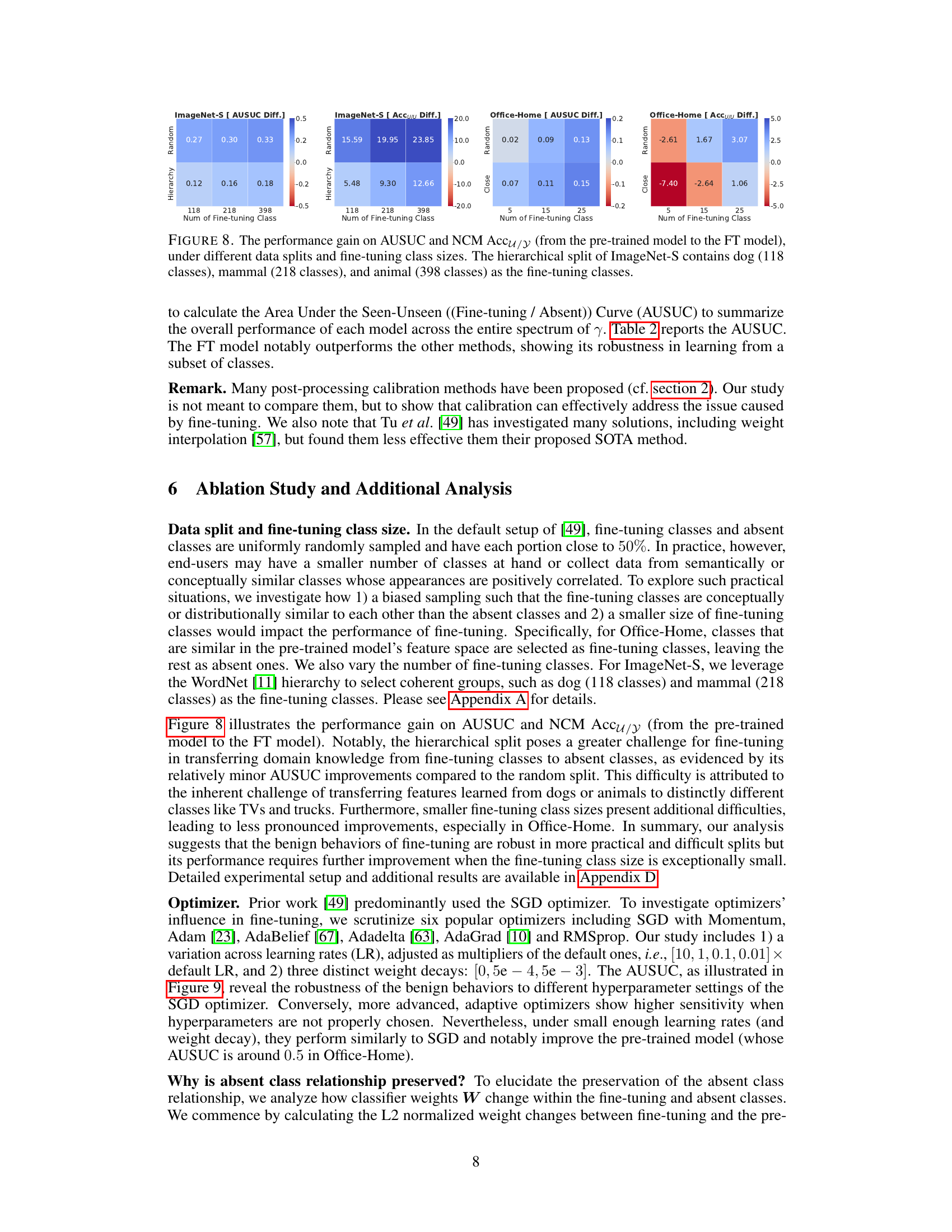
This figure compares the accuracy gain on fine-tuning and absent classes after fine-tuning using two different classifiers: a neural network (NN) classifier and a Nearest Class Mean (NCM) classifier. The NN classifier shows a decrease in accuracy for absent classes, while the NCM classifier shows an increase, indicating an overall improvement in feature extraction for all classes after fine-tuning. This suggests that fine-tuning with a subset of classes holistically improves the feature extractor for the downstream domain.

This figure compares the accuracy gain (or loss) after fine-tuning for both a neural network classifier and a Nearest Class Mean (NCM) classifier. The neural network uses the full architecture, including the fully connected layer, while the NCM classifier only uses the extracted features. The results show that while the neural network suffers an accuracy drop in the classes not seen during fine-tuning (absent classes), the NCM classifier shows a consistent gain across all classes. This highlights the improvement of features in the fine-tuned model, despite the loss of accuracy in the standard classifier.

This figure shows the relationship between the accuracy of classifying fine-tuning classes (Accs/y) and the accuracy of classifying absent classes (Accu/y) on the ImageNet-Variants dataset as the calibration factor γ is varied. The graph displays curves for the pre-trained model, the fine-tuned model, the fine-tuned model with post-processing calibration (Fine-tuning + γ), the state-of-the-art model from the paper by Tu et al. [49] , and the state-of-the-art model with calibration (Tu et al. 2023 + γ). The figure illustrates that post-processing calibration can significantly improve the accuracy on absent classes without significantly reducing accuracy on fine-tuning classes.

This figure compares the accuracy gain of neural network (NN) and nearest class mean (NCM) classifiers after fine-tuning. The NN classifier shows accuracy drops for absent classes, while the NCM classifier shows accuracy gains for absent classes. This indicates that fine-tuning improves feature representation for all classes but the NN classifier is unable to fully leverage the improved features due to a calibration issue.
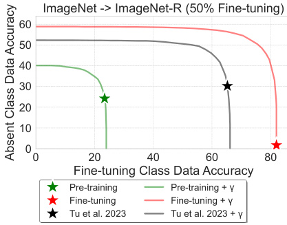
This figure shows the absent class accuracy (Accu/y) plotted against the fine-tuning class accuracy (Accs/y) for the ImageNet-R dataset with 50% of classes used for fine-tuning. The different colored lines represent different methods: the pre-trained model (green star), the fine-tuned model (red star), the state-of-the-art method from Tu et al. 2023 (black star), and the calibrated versions of each using the bias factor γ (colored lines). The plot illustrates the impact of calibration in restoring the accuracy of the model on absent classes (as Accu/y increases with the calibration).

This figure shows the accuracy gain (difference between the accuracy after fine-tuning and the accuracy of the pre-trained model) of both NN and NCM classifiers for fine-tuning and absent classes after fine-tuning on three different datasets: ImageNet-{R,S}, VTAB, and Office-Home. The NN classifier shows decreased accuracy for absent classes, indicating negative transfer, while the NCM classifier shows improved accuracy for absent classes, suggesting holistic feature improvement by fine-tuning. This highlights that the issue with absent classes is not feature degradation but a different problem (logit scale discrepancy).
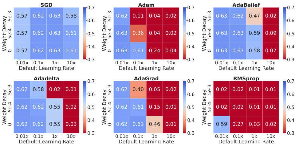
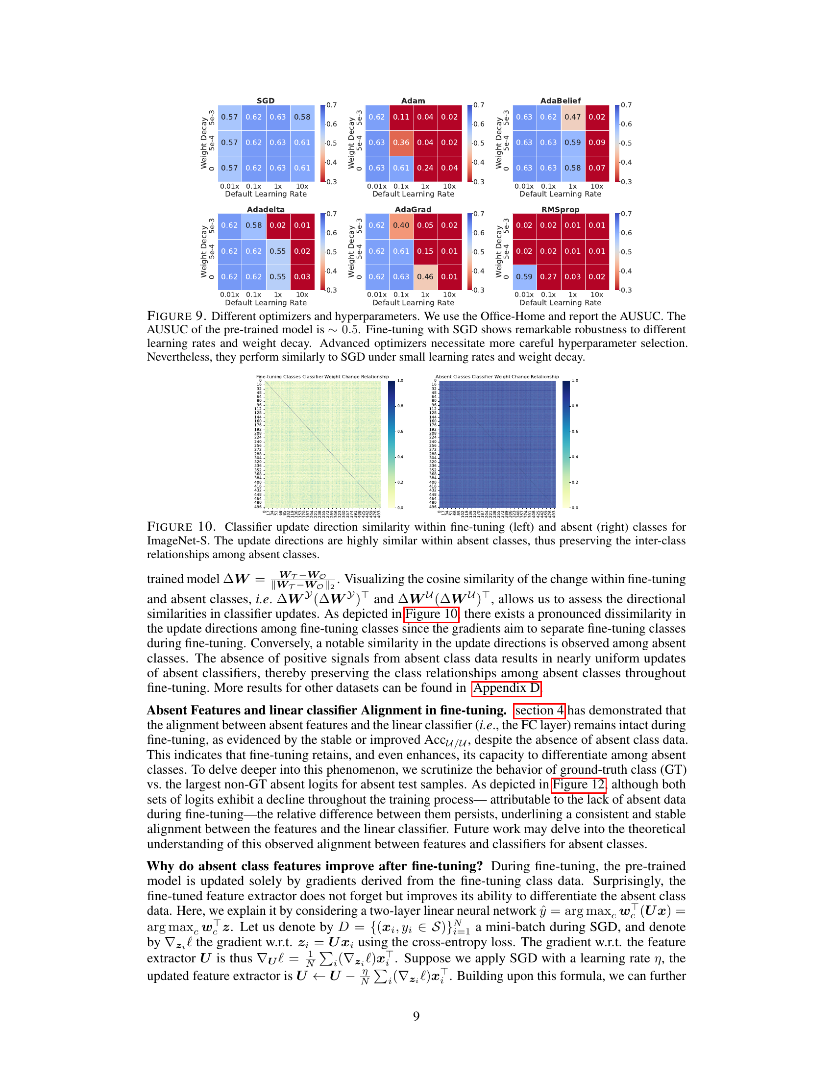
This figure shows the AUSUC (Area Under the Seen-Unseen Curve) for different optimizers (SGD, Adam, AdaBelief, Adadelta, AdaGrad, RMSprop) and hyperparameter settings (learning rates and weight decay) on the Office-Home dataset. It demonstrates the robustness of the SGD optimizer to variations in hyperparameters, while showing the increased sensitivity of other, more advanced optimizers, especially when hyperparameters are not carefully tuned. Even with the more advanced optimizers, comparable performance to SGD can be achieved with smaller learning rates and weight decay.
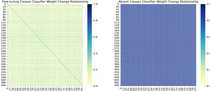
This figure visualizes the cosine similarity of the changes in classifier weights (the difference between weights after and before fine-tuning) for both fine-tuning and absent classes in ImageNet-S. The high similarity of update directions within the absent classes shows that the relationships between these classes are preserved during fine-tuning, despite the absence of absent class data during the fine-tuning process.

This figure shows two plots. The left plot is a scatter plot visualizing the movement of features for fine-tuning and absent classes before and after fine-tuning. The right plot is a line graph showing the average logits for ground-truth absent classes and the largest non-ground-truth absent class logits over training epochs. Both plots demonstrate that the fine-tuning process maintains a stable relationship between features and linear classifiers, even for absent classes.
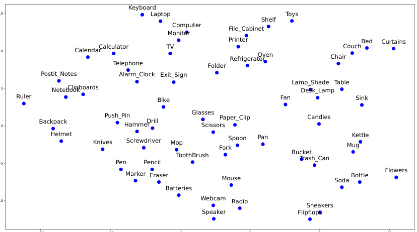
This figure illustrates the concept of fine-tuning a pre-trained model. The pre-trained model is initially trained on a large dataset (e.g., ImageNet), encompassing a wide range of classes. Fine-tuning then adapts this model to a specific downstream task using a smaller dataset that only includes a subset of the original classes. The figure highlights a crucial point: while the fine-tuned model excels at the classes present in the downstream dataset, its performance on unseen classes (those not part of the downstream dataset but present in the initial pre-training dataset) can significantly decrease. This demonstrates the risk of losing valuable knowledge previously learned during pre-training when fine-tuning is not carefully calibrated.

This figure compares the accuracy gain (difference between fine-tuned and pre-trained model accuracy) for fine-tuning classes and absent classes using two classifiers: a neural network classifier (NN) and a Nearest Class Mean classifier (NCM). The NN classifier shows a decrease in accuracy for absent classes after fine-tuning, while the NCM classifier shows improvement, indicating that feature extraction is not degraded, and potentially even enhanced, by fine-tuning.
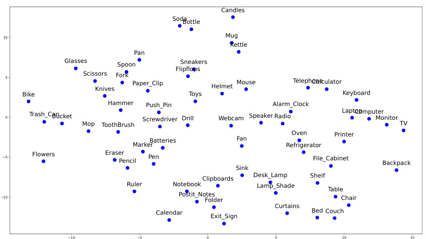
This figure illustrates the process of fine-tuning a pre-trained model. The pre-trained model is initially trained on a large dataset (e.g., ImageNet). This model is then fine-tuned on a smaller, more specific dataset for a downstream task. The key point highlighted is that, during deployment, the fine-tuned model might encounter new classes (absent classes) not present in the fine-tuning dataset. The ideal outcome is that the fine-tuned model performs well on both the fine-tuning classes and the unseen classes.

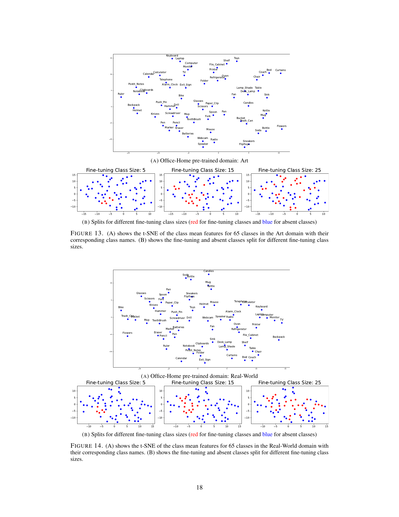
This figure visualizes the feature distribution of classes using t-SNE in the Art domain of the Office-Home dataset and how the classes are split into fine-tuning and absent classes for different fine-tuning class sizes. Panel A shows the t-SNE visualization of the class mean features. Panel B illustrates the different splits for various fine-tuning sizes, where red points represent fine-tuning classes and blue points represent absent classes.
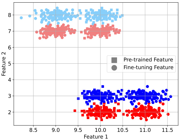
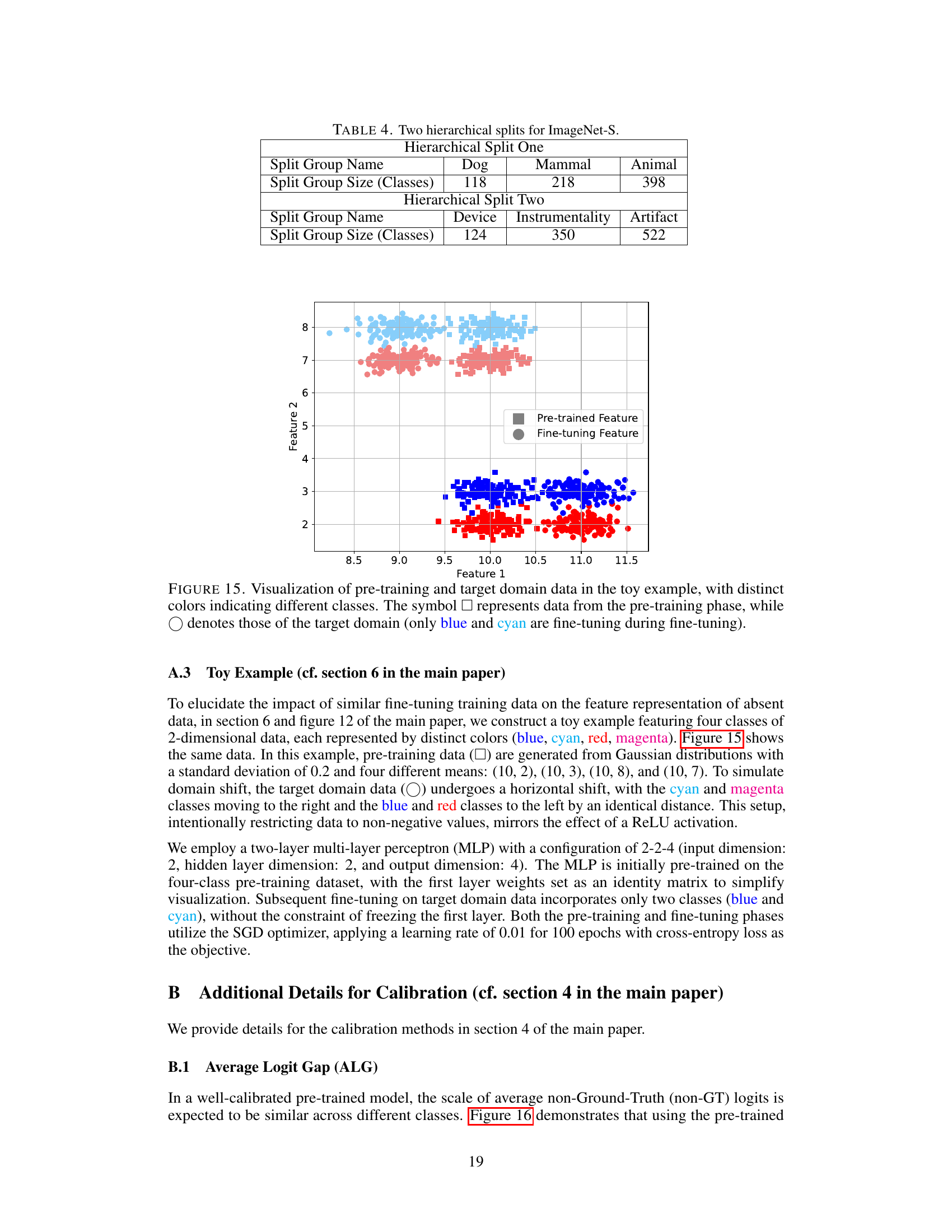
This figure shows the visualization of pre-training data and target domain data for a toy example with four classes. The pre-training data is represented by squares (□) and target domain data is represented by circles (○). The colors represent different classes, with blue and cyan representing the fine-tuning classes during fine-tuning. The figure helps illustrate the effect of fine-tuning on the feature representation of the data in different domains.
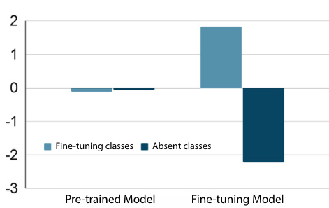
This figure compares the accuracy gain of neural network (NN) classifier and Nearest Class Mean (NCM) classifier after fine-tuning. The results show that the NN classifier’s accuracy on absent classes decreases while NCM classifier’s accuracy increases. This suggests that the features extracted by the fine-tuned model are improved holistically, even for those classes not included in the fine-tuning process.

This figure illustrates the Average Logit Gap (ALG) method for calibrating the logits of a fine-tuned model. It shows how the calibration factor (γ) is calculated using the difference between the average non-ground-truth (non-GT) logits of the fine-tuning classes and the average non-GT logits of the absent classes in the training data. This difference is used to adjust the logits of the absent classes, aiming to bring their magnitude closer to the logits of the fine-tuning classes.
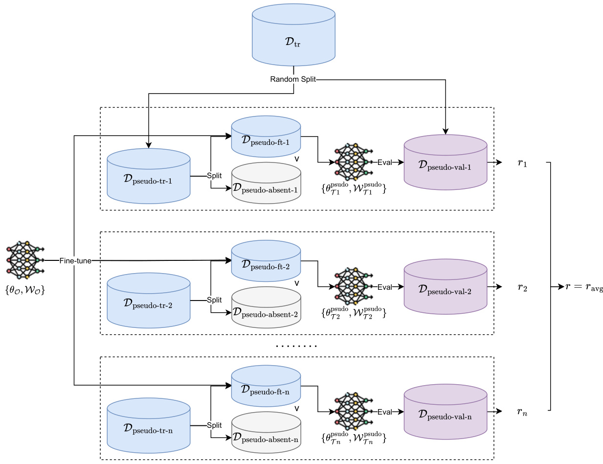
This figure illustrates the Pseudo Cross-Validation (PCV) method used in the paper to estimate the calibration factor gamma (γ). The method involves repeatedly splitting the training data into pseudo-fine-tuning and pseudo-absent sets. A fine-tuned model is trained on each pseudo-fine-tuning set, and its performance is evaluated on the corresponding pseudo-validation set. The average of the resulting performance metrics is used to select the final value of γ.
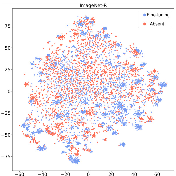
This figure shows the t-SNE visualization of ImageNet-R dataset’s features extracted by the fine-tuned model. The visualization demonstrates that the fine-tuned feature extractor does not create a clear separation between the fine-tuning and absent classes in the feature space, indicating that the model does not simply learn to discriminate between them by creating a large margin, but rather uses a more nuanced and holistic representation of the data.
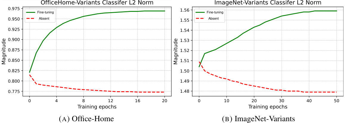
This figure shows the L2 norm of classifier weights for fine-tuning and absent classes during fine-tuning. The plots illustrate that the magnitude of the weights for fine-tuning classes increases significantly more than that of absent classes. This suggests that the fine-tuning process disproportionately boosts the importance of fine-tuning classes, leading to the observed bias in logit predictions towards those classes.
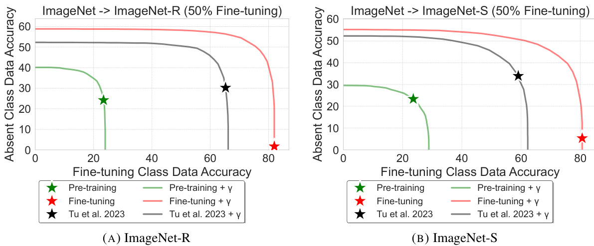
This figure shows the accuracy of classifying fine-tuning classes (Accs/y) and absent classes (Accu/y) for different calibration factors (γ) on ImageNet-R and ImageNet-S. The x-axis represents the accuracy on fine-tuning classes, and the y-axis represents the accuracy on absent classes. The lines show the performance of pre-training, fine-tuning (without calibration), fine-tuning with calibration, and the state-of-the-art model from Tu et al. 2023, both with and without calibration. This figure demonstrates that post-processing calibration can effectively restore the accuracy on absent classes that is lost during fine-tuning.

This figure shows the absent class accuracy (Accu/y) versus fine-tuning class accuracy (Accs/y) curves for all six combinations of source and target domains in the Office-Home dataset. Each curve represents a different source-target domain pair. The curves demonstrate the impact of the proposed post-processing calibration method (adding a bias factor γ to the logits of absent classes) on both Accu/y and Accs/y. The results show that calibration improves absent class accuracy while maintaining reasonably good fine-tuning class accuracy.

This figure shows the performance of the fine-tuning model with post-processing calibration on the VTAB dataset. The x-axis represents the accuracy on the fine-tuning classes (Accs/y), and the y-axis represents the accuracy on the absent classes (Accu/y). Each subfigure represents a different dataset within VTAB, showing how the calibration factor improves the accuracy on absent classes while maintaining reasonable accuracy on the fine-tuning classes. The results are compared to the pre-trained model and the model fine-tuned without calibration, highlighting the effectiveness of the proposed method.

This figure shows the accuracy gain in both fine-tuning and absent classes after fine-tuning. Two classifiers are used: a neural network classifier with a fully connected layer and a nearest class mean (NCM) classifier using only features. The results demonstrate that the NCM classifier shows an improvement in accuracy for absent classes, while the neural network classifier exhibits a drop in accuracy for absent classes. This highlights that the fine-tuning process leads to improved feature extraction for all classes, even those not included in the fine-tuning process.

This figure shows the accuracy gain for fine-tuning classes and absent classes after fine-tuning using two types of classifiers: Neural Network (NN) classifier and Nearest Class Mean (NCM) classifier. The NN classifier shows an accuracy drop for absent classes, while the NCM classifier shows a consistent accuracy gain, indicating an overall improvement in feature quality after fine-tuning. This suggests that fine-tuning with only a subset of classes can improve the feature extractor for all classes, including those not seen during fine-tuning.

This figure compares the accuracy gain after fine-tuning using two different classifiers: a neural network (NN) classifier and a Nearest Class Mean (NCM) classifier. The NN classifier shows an accuracy drop for the absent classes after fine-tuning, while the NCM classifier shows a consistent gain, indicating that the quality of the extracted features improves holistically after fine-tuning, even for the classes not included during fine-tuning.

This figure visualizes the cosine similarity of the change in classifier weights between fine-tuning and the pre-trained model for both fine-tuning and absent classes in ImageNet-S. The high similarity in update directions for absent classes indicates that the relationships between these classes are preserved during fine-tuning, even though they weren’t directly involved in the training process.

This figure shows a visualization of the data used in a toy example to illustrate the impact of similar fine-tuning training data on the feature representation of absent data. The pre-training data is represented by squares (□) and the target domain data by circles (○). The colors of the circles represent different classes. Only the blue and cyan circles are used in the fine-tuning process.
More on tables
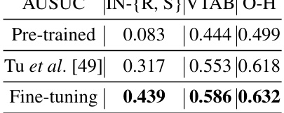
This table presents the Area Under the Seen-Unseen Curve (AUSUC) for three different methods: Pre-trained, Tu et al. [49], and Fine-tuning, across three benchmark datasets: ImageNet-{R, S}, VTAB, and Office-Home. AUSUC is a metric used to evaluate the performance of fine-tuning models on both seen and unseen classes. The higher the AUSUC, the better the model’s performance. The results show that fine-tuning achieves better results than the other two methods across all three datasets.
This table presents the results of post-processing calibration experiments on various datasets. It shows the accuracy (Acc) of classifying both fine-tuning and absent classes, comparing the performance of the pre-trained model, the fine-tuned model, and the fine-tuned model with post-processing calibration applied using different methods. The ‘Oracle’ row represents an upper bound, where the model is trained with both fine-tuning and absent class data. The results demonstrate that post-processing calibration effectively improves the accuracy on absent classes, often achieving performance comparable to or exceeding the state-of-the-art (SOTA) methods that use more complex training strategies.

This table presents the performance comparison of different methods in terms of accuracy on fine-tuning classes and absent classes. The methods include a pre-trained model, fine-tuning, fine-tuning with post-processing calibration using different approaches (ALG, PCV, and an oracle method), and a state-of-the-art method from previous research. The results are shown for different datasets: ImageNet-{R,S}, VTAB, and Office-Home. The ‘Oracle’ row shows the upper bound performance achievable if the model was trained with both fine-tuning and absent classes.

This table compares the performance of two classifiers: a neural network (NN) classifier with a fully connected (FC) layer and a cosine classifier. The comparison is done using several metrics including AUSUC (Area Under the Seen-Unseen Curve), Accy/y (accuracy of classifying fine-tuning class data to all classes), Accs/y (accuracy of classifying fine-tuning class data to fine-tuning classes), and Accu/y (accuracy of classifying absent class data to all classes). The results show that both classifiers achieve similar performance on the ImageNet-Variants and Office-Home benchmarks. This suggests the importance of logit calibration on the final classifier weights.

This table presents the performance comparison of different methods on various datasets for image classification. The methods include: pre-trained model (no fine-tuning), fine-tuning only, a state-of-the-art (SOTA) method from a previous paper by Tu et al. [49], fine-tuning with post-processing calibration using ALG, fine-tuning with post-processing calibration using PCV, and an oracle approach (fine-tuning with both fine-tuning and absent classes). The metrics used to evaluate performance are Accuracy of fine-tuning classes (Accs/y), Accuracy of absent classes (Accu/y). The table demonstrates that post-processing calibration significantly improves the accuracy of classifying absent classes, recovering much of the performance lost during fine-tuning, and even outperforming the SOTA method in some cases. The oracle model represents an upper bound on performance, showing the potential for further improvement in the absence of full datasets.

This table presents a comparison of the Area Under the Seen-Unseen Curve (AUSUC) and the Nearest Class Mean accuracy (NCM Accu/y) for four different approaches: Pre-trained, Fine-Tuning, Frozen Classifier, and Linear Probing. The results show that the Fine-Tuning method outperforms the other three methods on both metrics. This indicates that simply fine-tuning all the model parameters is the most effective method for maintaining accuracy on both the fine-tuning classes and the absent classes, compared to freezing parts of the model (such as the classifier) or only updating a small subset of parameters (linear probing).

This table presents the results of post-processing calibration on several datasets. It shows the accuracy (Accs/y, Accu/y) of classifying fine-tuning and absent classes, both before and after fine-tuning, and after applying different calibration techniques. The ‘Pre-trained’ row shows the performance of the model before fine-tuning, while the ‘Fine-tuning’ row displays performance after standard fine-tuning. The remaining rows illustrate the results of the proposed calibration approaches, along with a comparison to the state-of-the-art (SOTA) method from a previous study. The ‘Oracle’ row provides an upper bound, representing performance that would be achieved if the model were trained with both fine-tuning and absent classes.

This table presents the performance comparison of different methods for fine-tuning a pre-trained model. It shows the accuracy (Acc) on fine-tuning classes and absent classes, separately. The ‘Pre-trained’ row shows the performance of the model before fine-tuning. The ‘Fine-tuning’ row represents the performance after fine-tuning without any calibration. The ‘Tu et al. [49]’ row shows the results obtained using the state-of-the-art (SOTA) method from a previous study. The rows with ‘Fine-tuning +…’ demonstrate the performance improvements achieved by applying post-processing calibration methods proposed in this paper (ALG, PCV, and y*). Finally, ‘Oracle’ represents the upper bound performance that can be theoretically achieved if the model were fine-tuned using both fine-tuning and absent class data. The metrics for each method (Pre-trained, Fine-tuning, Tu et al. [49], Fine-tuning + ALG, Fine-tuning + PCV, Fine-tuning + y*, Oracle) are shown for different datasets: ImageNet-{R,S}, VTAB, and Office-Home.

This table presents the performance comparison of different methods on various datasets (ImageNet-{R,S}, VTAB, Office-Home). It shows the accuracy (Acc) for fine-tuning classes and absent classes, both before and after post-processing calibration. The results demonstrate that a simple post-processing calibration can significantly improve the accuracy of the fine-tuned model on absent classes, effectively recovering the pre-trained model’s capabilities. The ‘Oracle’ row represents the upper bound performance achieved when the model is fine-tuned with both fine-tuning and absent class data.

This table presents the performance comparison between different methods for fine-tuning a pre-trained model and recognizing both fine-tuning classes and absent classes. The methods compared include the pre-trained model’s performance, fine-tuning only, the state-of-the-art (SOTA) method by Tu et al. [49], and fine-tuning with post-processing calibration using two different approaches (ALG and PCV). An ‘Oracle’ result shows the theoretical best performance achievable if the model was trained with both fine-tuning and absent class data. The results show the effectiveness of calibration methods in improving the accuracy on absent classes.

This table presents the performance of different methods on three benchmark datasets: ImageNet-{R, S}, VTAB, and Office-Home. The metrics shown are accuracy for fine-tuning classes (Accs/y), accuracy for absent classes (Accu/y), and overall accuracy (Accy/y). It demonstrates the effectiveness of post-processing calibration in recovering absent class accuracy after fine-tuning a pre-trained model with only a subset of classes. The ‘Oracle’ row represents the upper bound performance, achieved using fine-tuning with both fine-tuning and absent classes. The results show that using a simple post-processing calibration method significantly improves absent class accuracy compared to standard fine-tuning.

This table shows the performance comparison between the pre-trained model and the fine-tuned model on the iWildCam benchmark. The metrics compared include AUSUC (Area Under the Seen-Unseen Curve), Accy/y (accuracy of classifying fine-tuning class data), Accs/s (accuracy of classifying fine-tuning class data into fine-tuning classes only), Accu/y (accuracy of classifying absent class data), Accu/u (accuracy of classifying absent class data into absent classes only), NCM Accs/s (Nearest Class Mean accuracy of classifying fine-tuning class data using only features), and NCM Accu/y (Nearest Class Mean accuracy of classifying absent class data using only features). A negative value in the Δ row indicates a decrease in performance after fine-tuning, which was observed in the iWildCam benchmark.
Full paper#

