Continuous Product Graph Neural Networks

↗ OpenReview ↗ NeurIPS Homepage ↗ Chat

TL;DR

#

Key Takeaways

#

Why does it matter?

#

This paper is important because it introduces a novel and efficient method for processing multidomain data across multiple interacting graphs, a common challenge in various fields. CITRUS offers superior performance over existing approaches, opening new avenues for spatiotemporal forecasting and other applications involving multidomain graph data. Its theoretical analysis provides insights into stability and over-smoothing, contributing to a more robust understanding of continuous graph neural networks.

Visual Insights

#

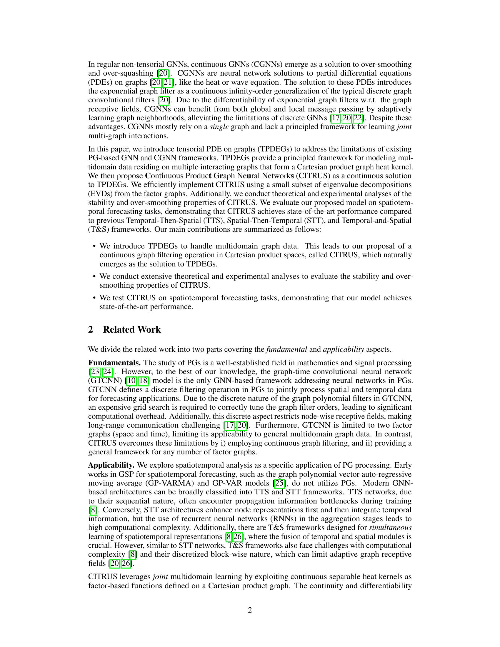
This figure illustrates the core concepts of the CITRUS model. Panel (a) shows a Cartesian product graph, which is a graph formed by combining multiple factor graphs (in this case, three). Each factor graph represents a different domain of data. Panel (b) demonstrates how the continuous product graph function (CITRUS) operates on multi-domain graph data (represented by U). The function uses continuous heat kernels on each factor graph, and the combination of these kernels is what gives the CITRUS model its ability to perform efficient multi-domain graph learning. The figure shows how the multi-domain graph data is transformed by a continuous function that takes into account the interactions between different domains.

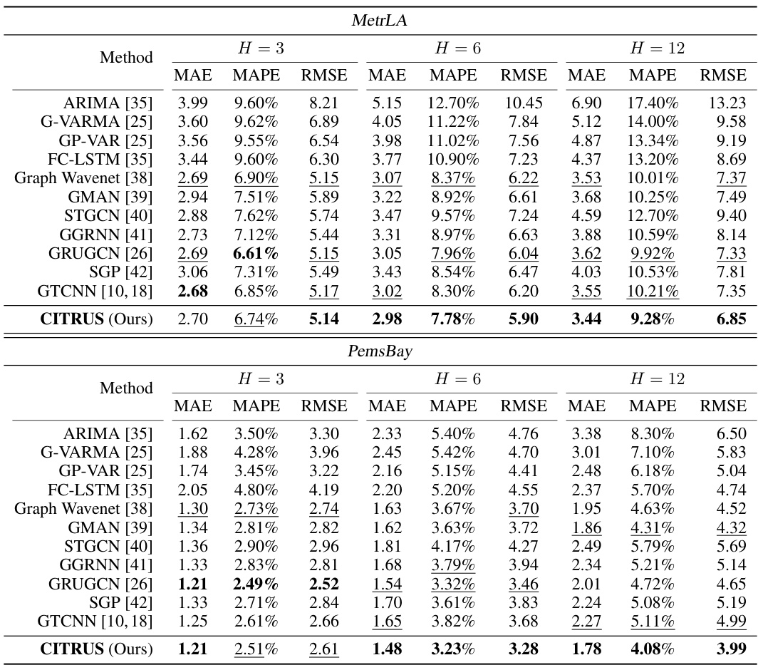
This table presents a comparison of the performance of CITRUS against other state-of-the-art methods on two benchmark traffic forecasting datasets (MetrLA and PemsBay). The comparison is made across three different prediction horizons (H=3, H=6, H=12), using three different metrics: Mean Absolute Error (MAE), Mean Absolute Percentage Error (MAPE), and Root Mean Squared Error (RMSE). The results show that CITRUS outperforms many existing methods in terms of accuracy and generalizability, especially for longer prediction horizons.

In-depth insights

#

Multi-graph Data

#

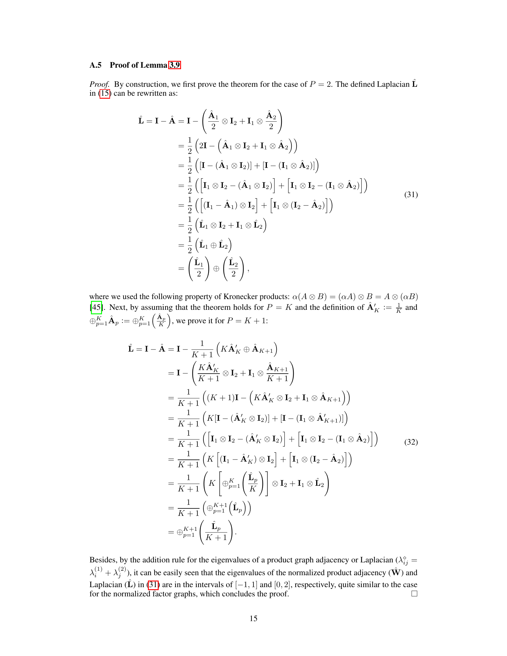
Multi-graph data, encompassing data distributed across multiple interconnected graphs, presents a significant challenge and opportunity in machine learning. The complexity arises from the need to model not only individual graph structures but also the intricate relationships between them. Current methods often simplify this by focusing on individual graphs or employing discrete operations, neglecting the continuous nature of many real-world interactions. A key insight is the potential of tensorial representations to effectively capture the multi-domain nature of multi-graph data. This allows for a principled mathematical framework to model interactions. Developing efficient algorithms that can handle the high dimensionality and complex dependencies inherent in multi-graph data is crucial for progress. This includes exploring continuous rather than discrete approaches, potentially leveraging the separability of kernels from Cartesian graph products for computational efficiency. The applications are vast, ranging from spatiotemporal forecasting (weather, traffic) to brain signal processing and recommendation systems. Further research should focus on robust methods, addressing issues like over-smoothing and stability in the face of noisy or incomplete data, and developing scalable algorithms for extremely large multi-graph datasets.

TPDE-based GNN

#

TPDE-based GNNs represent a novel approach to graph neural networks (GNNs) by leveraging the framework of tensorial partial differential equations (TPDEs). This approach offers several advantages. First, it moves beyond traditional discrete graph filtering, enabling the modeling of complex relationships in multi-domain data residing on multiple interacting graphs. Second, TPDE-based GNNs can naturally handle tensorial data, allowing for more comprehensive representation of information. The key innovation lies in the continuous nature of the TPDEs, which contrasts with discrete GNN methods. This leads to improved expressiveness, mitigating the over-smoothing and over-squashing problems encountered in discrete models. Stability and over-smoothing are crucial considerations, therefore, the theoretical analysis of TPDE-based GNNs is key to understanding its behavior. The stability analysis assesses the robustness of the model against graph perturbations, ensuring reliable performance in real-world applications, while over-smoothing analysis addresses the tendency for the model to lose fine-grained information during multiple iterations. The success of TPDE-based GNNs ultimately relies on the successful application of TPDEs to graph data. This involves careful formulation of the TPDEs to capture the essential characteristics of the problem and effective numerical methods to solve them.

CITRUS Stability

#

The stability analysis of CITRUS, a continuous product graph neural network, is crucial for its reliability and performance. The theoretical analysis demonstrates that CITRUS is robust against perturbations in the factor graphs that constitute the Cartesian product graph. The stability is proven to be separable across the factors. This separability is a key advantage of CITRUS as it reduces the complexity of the stability analysis. Empirical validation using synthetic data verifies the theoretical findings by showing that increasing the signal-to-noise ratio in factor graphs improves the overall stability of the predictions. This robustness to noisy data is a significant practical advantage, making CITRUS suitable for real-world applications with inherent uncertainties in data acquisition. The study further investigates the impact of different noise levels (SNRs) on stability, confirming the theoretical results and highlighting the practical benefits of this design in scenarios with varying data quality. Overall, the presented analysis provides strong evidence of CITRUS’s robustness and reliability.

Over-smoothing

#

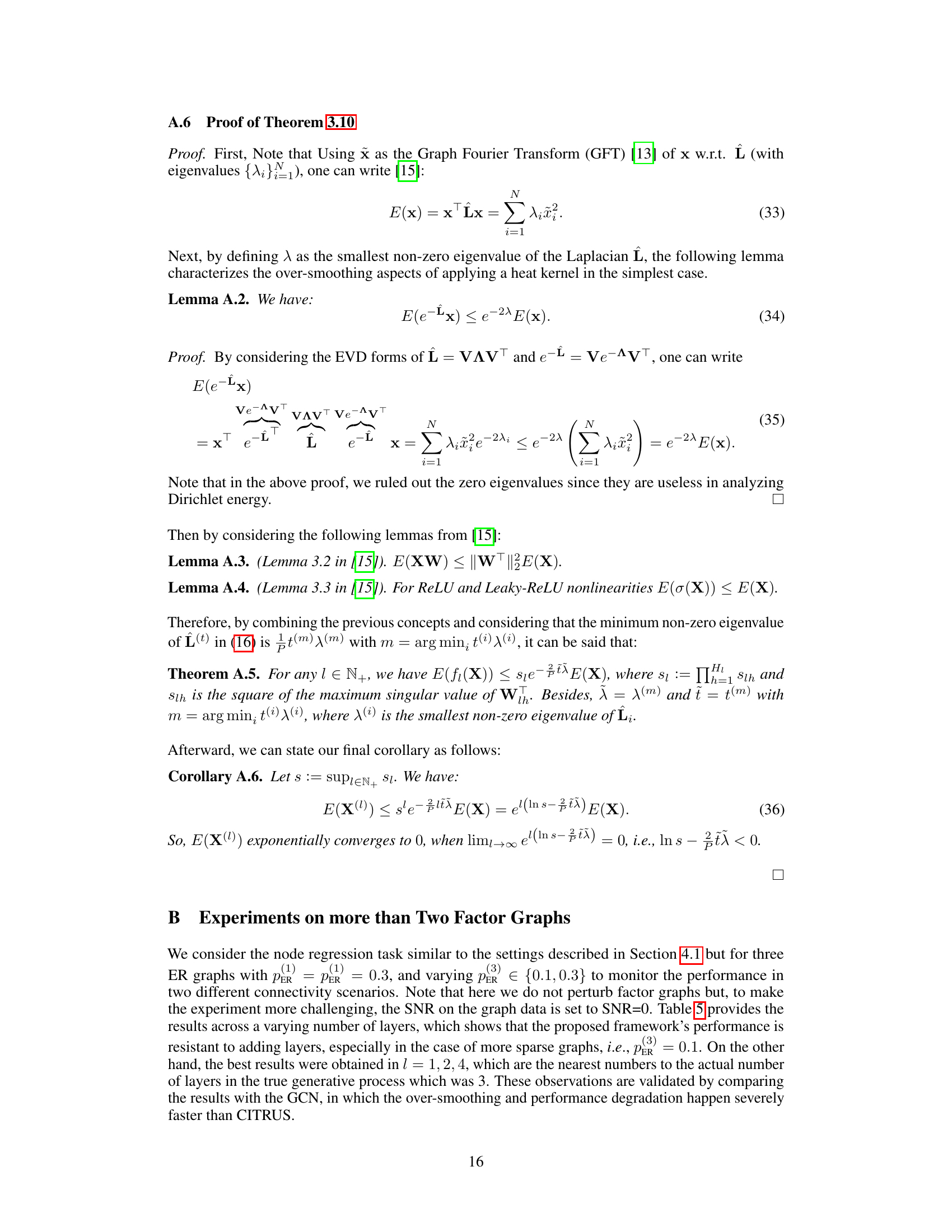
The concept of over-smoothing in graph neural networks (GNNs) is a critical challenge addressed in the paper. Over-smoothing occurs when the node representations in a GNN become too similar after multiple layers of aggregation, hindering the network’s ability to distinguish between nodes and learn complex relationships. The authors delve into the theoretical analysis of over-smoothing in the context of continuous GNNs (CGNNs) operating on Cartesian product graphs. They introduce a novel metric, Tensorial Dirichlet energy, to measure over-smoothing in multi-domain data, showing its connection to the spectral properties of the factor graphs. This enables understanding how over-smoothing depends on the spectral gap (difference between the smallest non-zero eigenvalue and zero) of individual factor graphs and the learnable receptive field of each layer. Their theoretical findings highlight the role of the smallest spectral gap in determining over-smoothing behavior and provide a framework for designing more robust and efficient GNN architectures. The paper further supports these theoretical results with empirical evidence, demonstrating how these insights translate into improved performance in practical applications.

Real-world Tests

#

A robust evaluation of any spatiotemporal forecasting model necessitates real-world testing. This involves applying the model to datasets representing genuine traffic flow or weather patterns, assessing its performance using metrics such as Mean Absolute Error (MAE), Mean Absolute Percentage Error (MAPE), and Root Mean Squared Error (RMSE). Real-world datasets often exhibit complexities not found in synthetic data, including noise, missing values, and non-stationary patterns, providing a more rigorous evaluation of the model’s generalization capabilities. Furthermore, the choice of datasets themselves is crucial; using well-established benchmarks like Metr-LA and PeMS-Bay for traffic forecasting, and Molene and NOAA for weather forecasting, adds credibility to the results. Benchmarking against state-of-the-art methods on these datasets allows for a direct comparison, enabling a fair assessment of the model’s performance. By reporting the results in such a manner, the paper would bolster confidence in the proposed model’s practical applicability and its potential for deployment in real-world scenarios. A comprehensive analysis, beyond simply reporting the numbers, would highlight the model’s strengths and weaknesses under different conditions and data characteristics. This would help in identifying its suitability for specific applications and future development directions.

More visual insights

#

More on figures

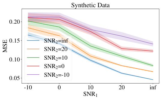
This figure shows the result of an experiment designed to test the stability of the CITRUS model against noise in the input data. The x-axis represents the signal-to-noise ratio (SNR) of the first factor graph, and the y-axis represents the mean squared error (MSE) of the model’s predictions. Different lines represent different SNR values for the second factor graph. The results show that the model’s performance improves as the SNR of both factor graphs increases, confirming the theoretical findings in Theorem 3.7.

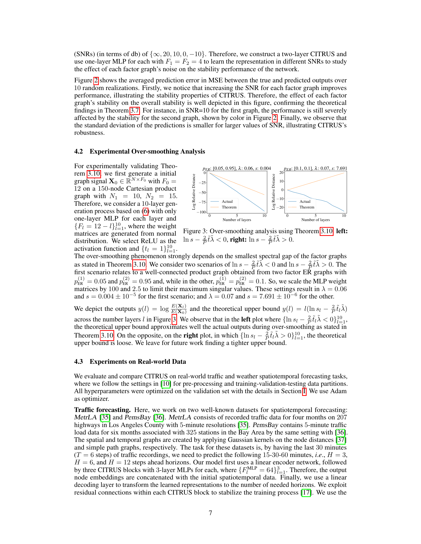
This figure shows the results of an experimental validation of Theorem 3.10, which concerns the over-smoothing analysis of the proposed CITRUS model. Two scenarios are presented: one where ln s − tx < 0 (left panel) and one where ln s − tx > 0 (right panel). The plots compare the actual log relative distance obtained from experiments to the theoretical upper bound given by the theorem, as a function of the number of layers in the model. The left panel demonstrates that the theoretical bound is a good approximation of the actual behavior when ln s − tx < 0, indicating the effectiveness of the theorem in predicting over-smoothing. In contrast, the right panel shows that the theoretical bound is less accurate when ln s − tx > 0, suggesting the need for a tighter theoretical upper bound in this case.

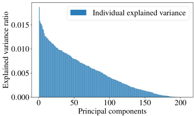
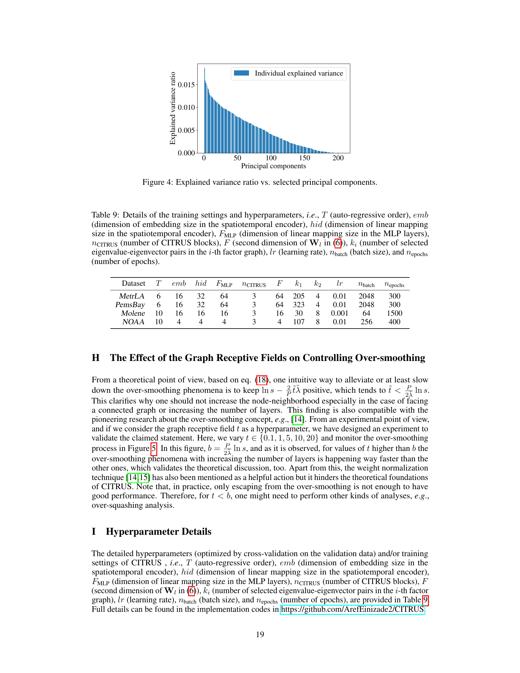
This figure shows the explained variance ratio plotted against the selected principal components of the spatial Laplacian for the MetrLA dataset. It demonstrates that a large portion of the variance is captured by a relatively small number of principal components, supporting the use of a low-rank approximation for computational efficiency in the proposed CITRUS method.

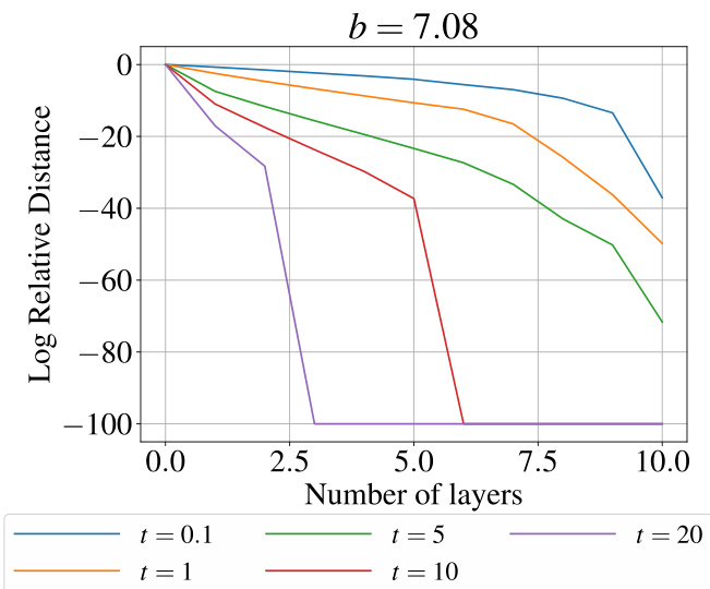
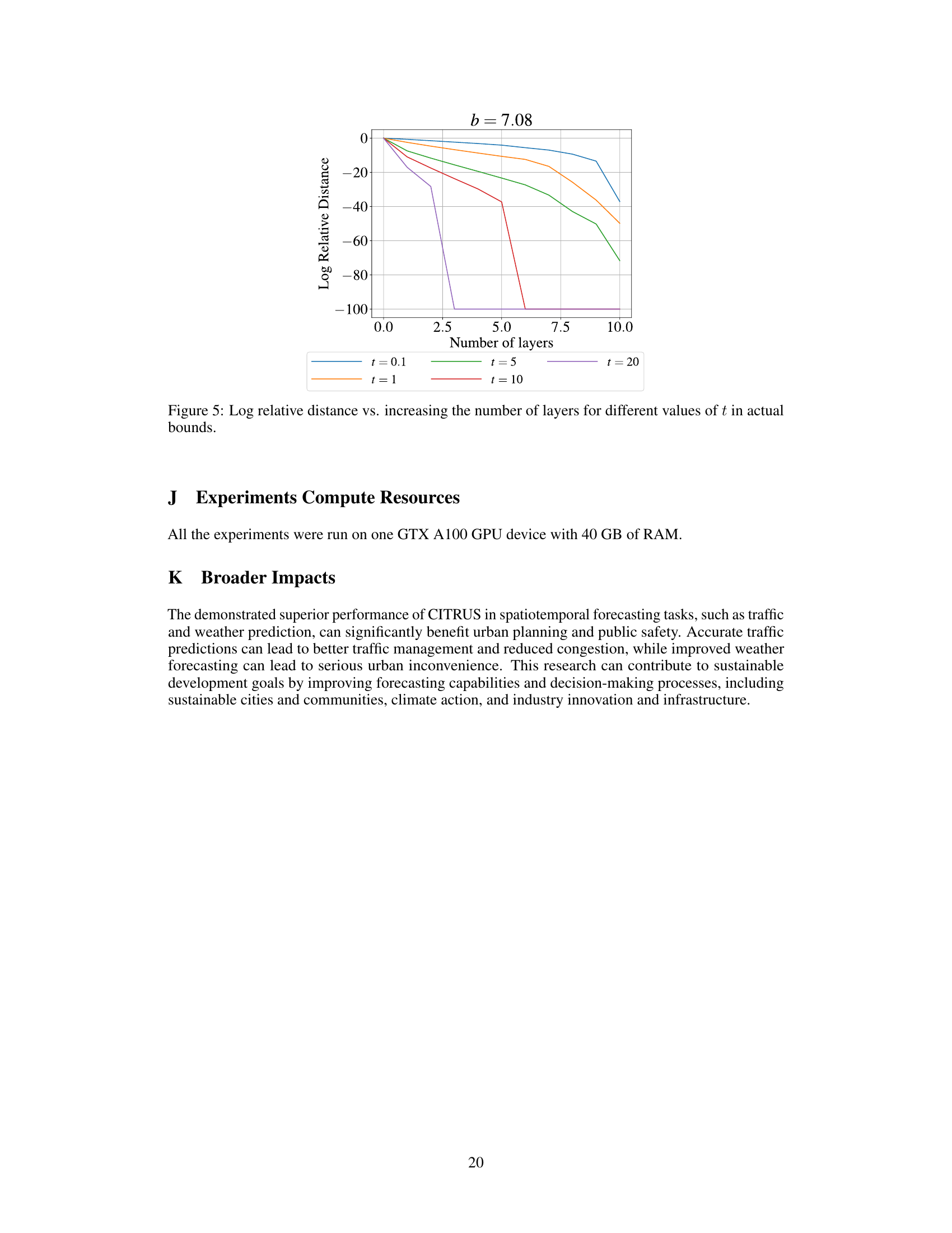
This figure shows the results of an experiment designed to validate the theoretical findings about over-smoothing in graph neural networks. The log relative distance is plotted against the number of layers for different values of the graph receptive field parameter, t. The plot illustrates how the rate of over-smoothing is affected by the choice of t, demonstrating that controlling the graph receptive field helps mitigate the issue of over-smoothing.

More on tables

This table presents the root normalized mean squared error (rNMSE) for weather forecasting using different methods on the Molene and NOAA datasets. The results are shown for different prediction horizons (H=1 to H=5), representing the number of hours into the future that the model is predicting. Lower rNMSE values indicate better forecasting accuracy. The table allows for a comparison of the proposed CITRUS model against other state-of-the-art methods in weather forecasting.

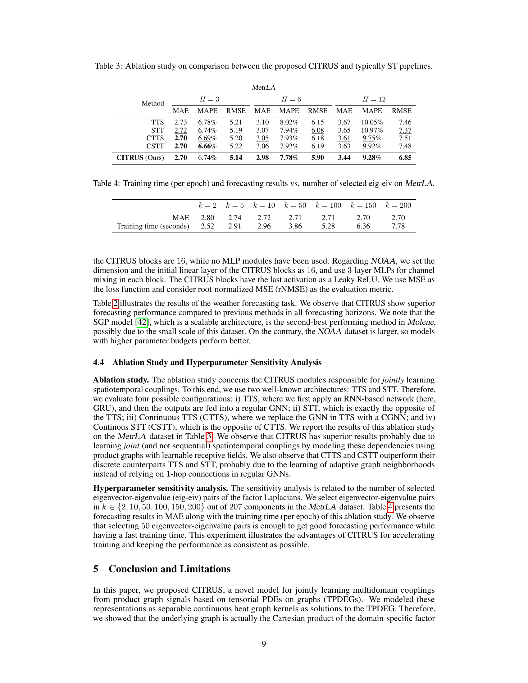
This table presents the ablation study comparing the proposed CITRUS model with other state-of-the-art methods such as TTS, STT, CTTS and CSTT. The performance metrics MAE, MAPE and RMSE are reported for different prediction horizons (H=3, H=6, H=12) on the MetrLA dataset. The results highlight CITRUS’s superior performance compared to other ST pipelines, demonstrating the effectiveness of its joint learning approach for spatio-temporal data.

This table presents the results of an ablation study on the effect of the number of selected eigenvector-eigenvalue pairs (k) on the performance of the CITRUS model for traffic forecasting on the MetrLA dataset. It shows the mean absolute error (MAE) and the training time per epoch for different values of k. The results indicate a trade-off between accuracy and computational cost, with diminishing returns in accuracy improvement as k increases.

This table presents the results of experiments conducted on more than two factor graphs. The node regression task is performed on three Erdős-Rényi factor graphs with varying edge probabilities to evaluate the model’s performance under different connectivity scenarios. The results are compared against a Graph Convolutional Network (GCN) baseline to highlight the effectiveness of the proposed CITRUS model in handling over-smoothing and maintaining performance even as the number of layers increases.

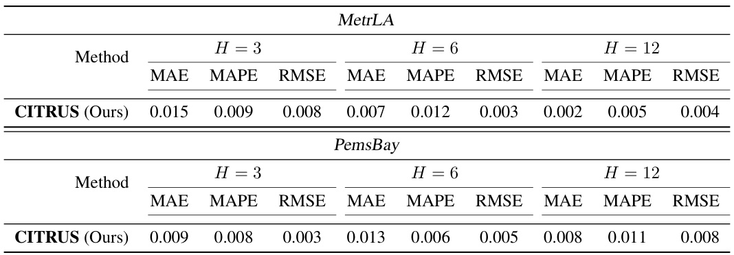
This table shows the standard deviation of the Mean Absolute Error (MAE), Mean Absolute Percentage Error (MAPE), and Root Mean Squared Error (RMSE) for the CITRUS model on the MetrLA and PemsBay datasets. The standard deviations are presented for different forecasting horizons (H=3, H=6, H=12). These values provide insight into the variability of the model’s predictions across different experimental runs.

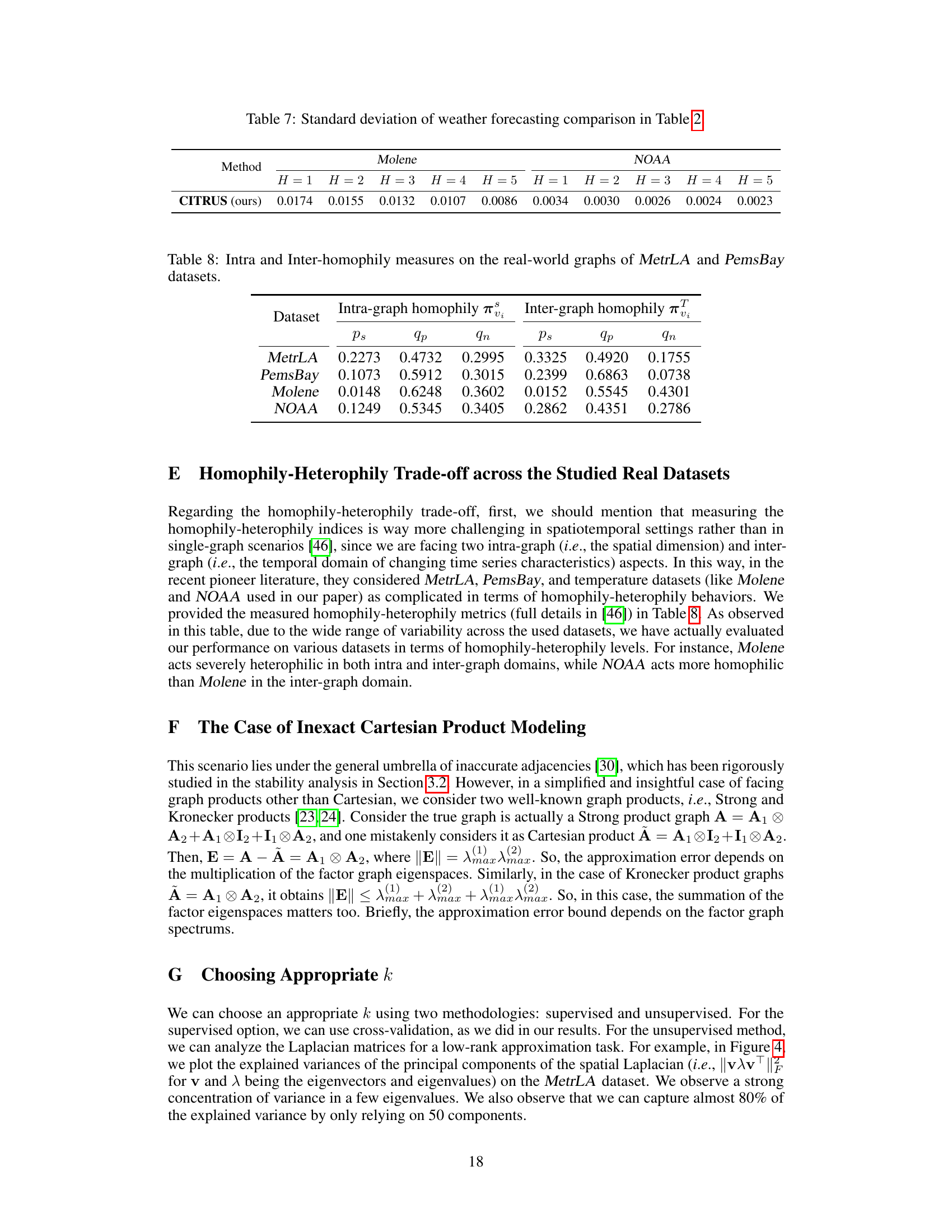
This table shows the standard deviation of the root normalized mean square error (rNMSE) for weather forecasting using the CITRUS model on the Molene and NOAA datasets. The results are broken down by prediction horizon (H) ranging from 1 to 5 hours.

This table presents the intra-graph and inter-graph homophily measures for four real-world datasets: MetrLA, PemsBay, Molene, and NOAA. Homophily refers to the tendency for nodes with similar characteristics to be connected. Intra-graph homophily measures the homophily within each individual graph (spatial graph), while inter-graph homophily measures homophily between the graphs (spatial-temporal correlation). Three metrics are used to quantify homophily: Ps: Pearson correlation between adjacency matrices and node attributes qP: The proportion of edges in the graph connecting node pairs with similar attributes qN: The number of neighbor pairs with the same attribute divided by the total number of pairs. This table provides quantitative insights into the degree of homophily and heterophily within and between the graphs of each dataset, showing significant variability across them.

This table shows the hyperparameters used in the experiments for different datasets. It includes parameters related to the autoregressive order, embedding dimensions, number of layers in MLPs and CITRUS blocks, number of selected eigenvectors, learning rate, batch size, and number of epochs.

Full paper

#