↗ OpenReview ↗ NeurIPS Homepage ↗ Chat
TL;DR#
Many real-world applications involve comparing datasets with different data types, creating heterogeneous joint distributions. Existing methods like Sliced Wasserstein (SW) and Generalized Sliced Wasserstein (GSW) fall short in handling this complexity, limiting their use. These methods efficiently compare distributions by projecting them onto one dimension, but they only work on homogeneous domains, which means all aspects of the data have to be similar. This limits their applicability to diverse data types.
This paper introduces a new method called Hierarchical Hybrid Sliced Wasserstein (H2SW), designed to tackle the problem. It uses a novel slicing method that deals with heterogeneous data by separating and then combining information from different data types. The authors extensively test H2SW on several applications like comparing 3D meshes, showing better performance than existing methods. They also provide detailed theoretical analysis of the method, proving that it is a valid metric and is computationally efficient.
Key Takeaways#
Why does it matter?#
This paper is crucial for researchers working with heterogeneous joint distributions, a common challenge in various fields. It offers a scalable and efficient solution to compare these complex datasets, which is vital for making meaningful comparisons across diverse data types. The proposed metric, H2SW, opens new avenues for research in areas like 3D mesh processing and deep learning, improving the accuracy and effectiveness of existing methods. Its theoretical properties are rigorously proven, which enhances its reliability and provides a solid foundation for future advancements.
Visual Insights#
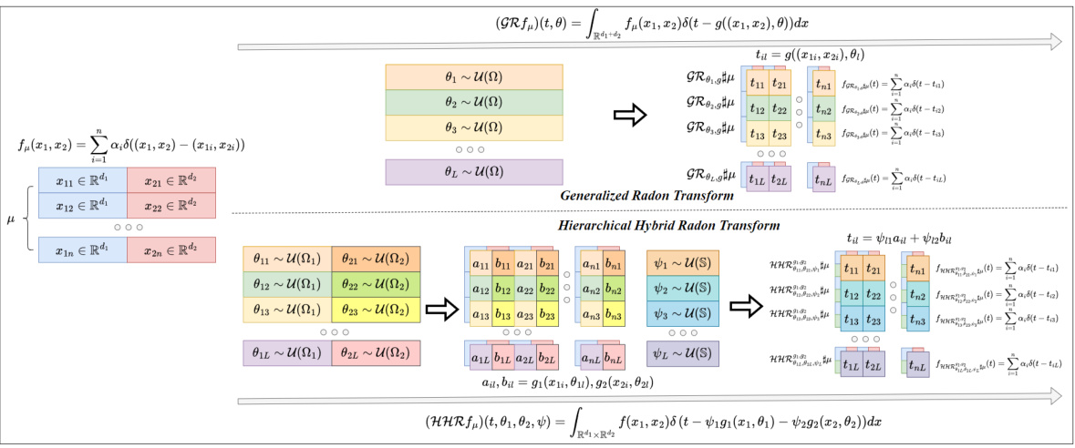
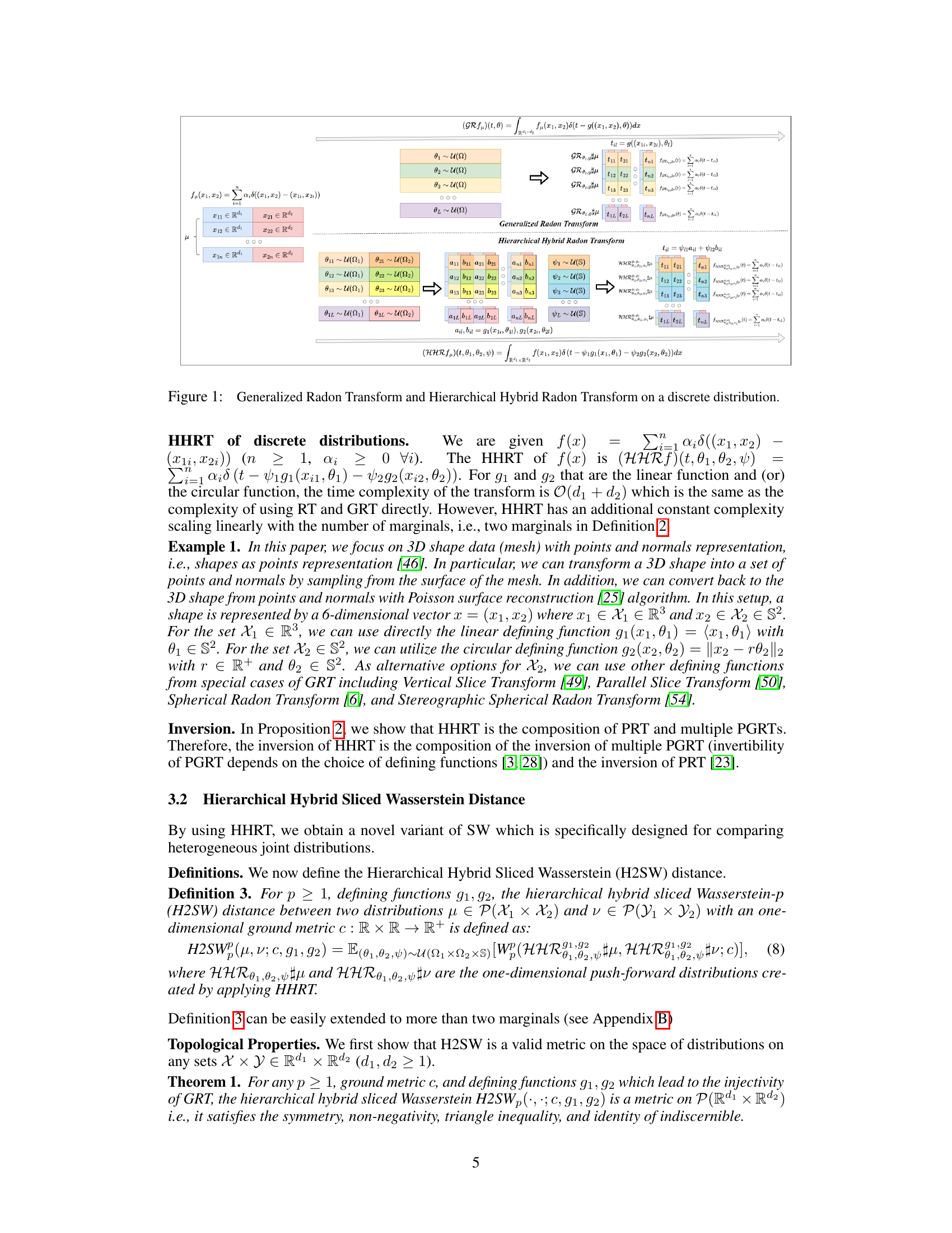
This figure illustrates the Generalized Radon Transform (GRT) and the Hierarchical Hybrid Radon Transform (HHRT) applied to a discrete distribution. The GRT shows a linear projection, while HHRT demonstrates a hierarchical approach. First, partial generalized Radon transforms (PGRT) with different defining functions are applied to each marginal argument. Then, a partial Radon transform (PRT) is applied to the joint transformed arguments to integrate information across marginals. This highlights the key difference between GRT’s linear projection and HHRT’s more expressive, hierarchical approach, which is better suited for handling heterogeneous joint distributions.

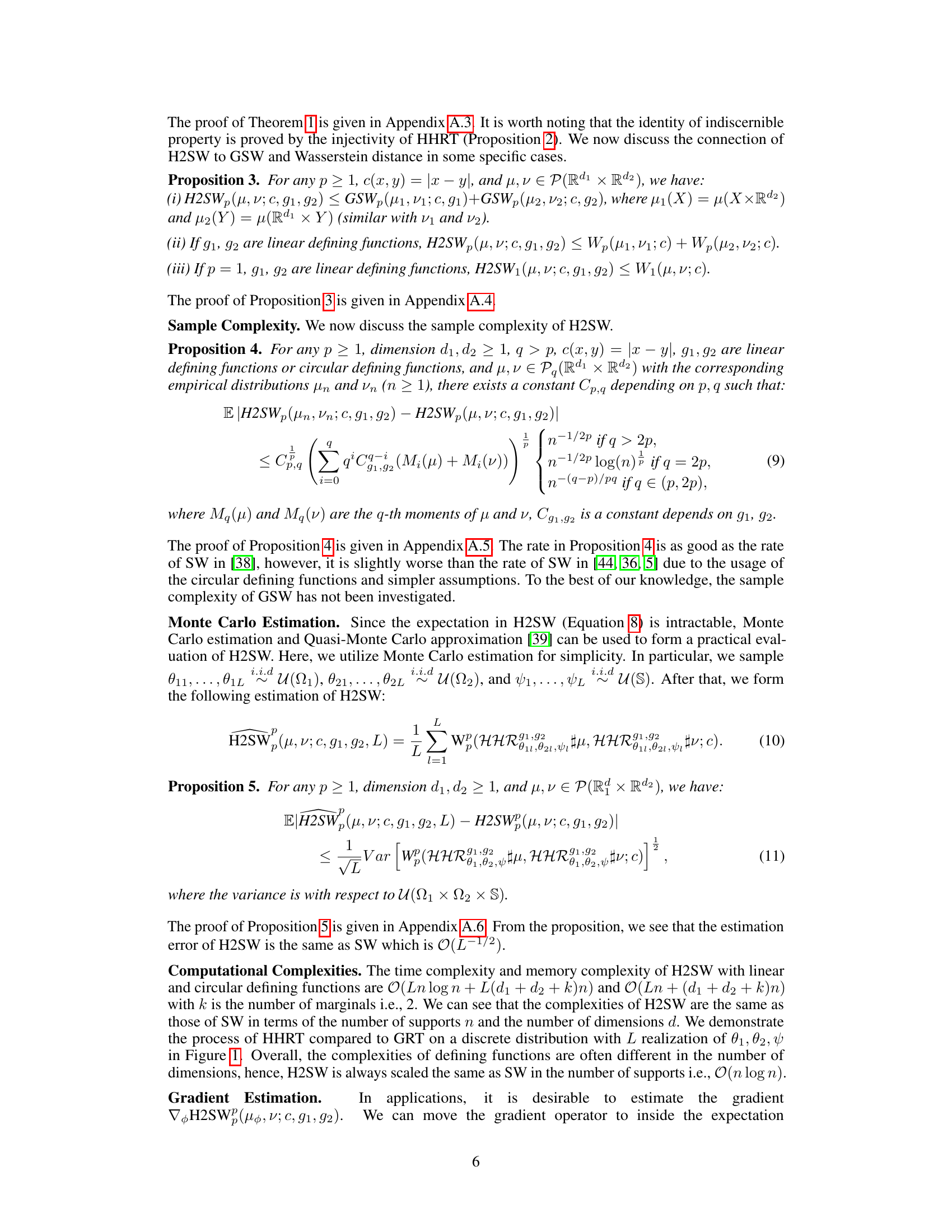
This table presents a quantitative comparison of three different methods (SW, GSW, and H2SW) for measuring the distance between meshes during a deformation process from a sphere mesh to an armadillo mesh. The comparison is done across various time steps (100, 300, 500, 1500, 4000, 5000), and for each method, two different numbers of projections (L=10 and L=100) are used. The results are presented as the mean ± standard deviation of the joint Wasserstein distance calculated for each method and parameter setting.
In-depth insights#
H2SW: A New Metric#
The proposed H2SW metric offers a scalable solution for comparing heterogeneous joint distributions, a significant advancement over existing methods like SW and GSW. Addressing the limitations of prior techniques restricted to homogeneous domains, H2SW leverages a novel Hierarchical Hybrid Radon Transform (HHRT) to effectively capture the structure of heterogeneous joint supports. This innovative approach enables meaningful comparisons across diverse marginal distributions. The topological and statistical properties of H2SW are rigorously examined, establishing its validity as a metric and demonstrating its favorable performance in several applications. The computational efficiency of H2SW, comparable to SW and GSW, makes it a practical and powerful tool for various machine learning, statistics, and data science applications. Future work should explore its extension to even more complex heterogeneous distributions and investigate its potential impact on a broader range of problems.
HHRT: Novel Slicer#
The heading “HHRT: Novel Slicer” suggests a significant contribution to the field of optimal transport. HHRT, likely an acronym for a novel Hierarchical Hybrid Radon Transform, presents a new approach to compute Wasserstein distances, a crucial metric in comparing probability distributions. The use of the term “slicer” implies that this transform projects high-dimensional data onto lower dimensions for efficient computation, overcoming limitations of existing methods like SW (Sliced Wasserstein) which struggle with heterogeneous data. This “novel slicer” potentially offers enhanced expressiveness in handling joint distributions with marginals supported on different domains by using a hierarchical approach, leading to a more accurate and scalable distance computation. The scalability and efficiency are crucial advantages as traditional Wasserstein distance calculation is computationally expensive. The effectiveness of this novel technique is further validated by its applicability in various applications such as 3D mesh deformation, deep mesh autoencoders, and datasets comparison, demonstrating a substantial advancement in the field.
3D Mesh Experiments#
The 3D mesh experiments section would likely detail the application of the proposed Hierarchical Hybrid Sliced Wasserstein (H2SW) distance to 3D mesh deformation tasks. This likely involved comparing H2SW against established methods like Sliced Wasserstein (SW) and Generalized Sliced Wasserstein (GSW). Key aspects to analyze would be how H2SW handles the heterogeneous nature of joint distributions inherent in 3D meshes (combining point cloud and surface normal data). The results might show improved accuracy or computational efficiency compared to baseline methods. The authors probably showcase this through quantitative metrics such as the joint Wasserstein distance itself and qualitative visualization of the mesh deformation process. A critical analysis should explore if H2SW offers advantages in scenarios with significant mesh complexity or non-uniform sampling density, and whether these advantages outweigh any potential increase in computational cost.
Autoencoder Results#
Autoencoder results would ideally present a quantitative evaluation of the model’s performance on reconstructing 3D mesh data. Key metrics would include joint Wasserstein distance, comparing the original and reconstructed meshes. Lower distances indicate better reconstruction quality. Qualitative results (visualizations) are also critical, showing examples of reconstructed meshes alongside their originals to assess visual fidelity. The impact of hyperparameters, specifically the number of projections (L), on both quantitative and qualitative results should be analyzed. Comparison to other autoencoders using traditional distance metrics would strengthen the findings, demonstrating the advantages of the proposed H2SW metric. A thorough analysis would also consider the computational efficiency of the autoencoder trained with H2SW versus baselines, particularly concerning training time and memory usage. Statistical significance of any observed improvements should be rigorously established.
Future Directions#
Future research could explore extending Hierarchical Hybrid Sliced Wasserstein (H2SW) to handle even more complex data structures, such as those involving time series or graph data. Investigating the theoretical properties of H2SW under different choices of slicing distributions and defining functions would provide deeper insights. The development of more efficient algorithms for computing H2SW is crucial for its broader application to large-scale datasets. Furthermore, exploring the use of H2SW in other machine learning tasks, beyond those studied in the paper (mesh deformation, autoencoders, and dataset comparison), could reveal its full potential. Finally, a detailed comparison of H2SW with other state-of-the-art metrics for heterogeneous data could solidify its position as a powerful tool for comparing complex distributions.
More visual insights#
More on figures
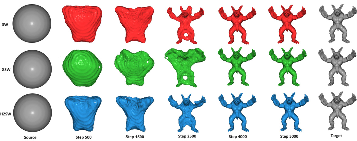
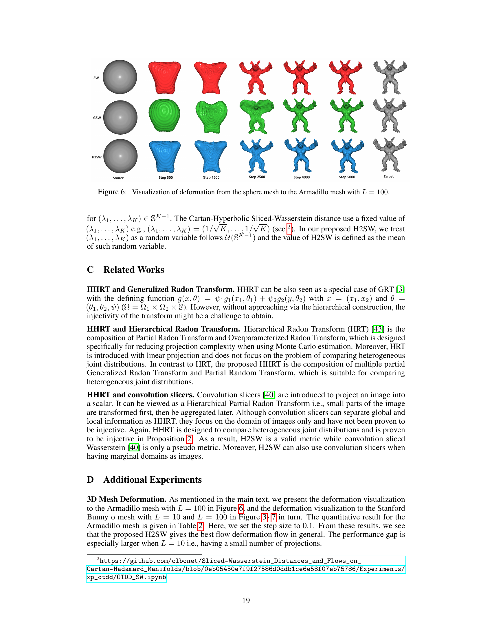
This figure visualizes the process of deforming a sphere mesh into an Armadillo mesh using three different Wasserstein distance methods: SW, GSW, and H2SW. Each row represents a different method, showing the intermediate steps of the deformation process from the source sphere mesh to the target Armadillo mesh. The parameter L, representing the number of projections, is set to 10. The images show how the shape evolves across time steps (500, 1500, 2500, 4000, and 5000), demonstrating the difference in deformation paths and convergence speed produced by the three algorithms.
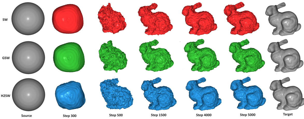
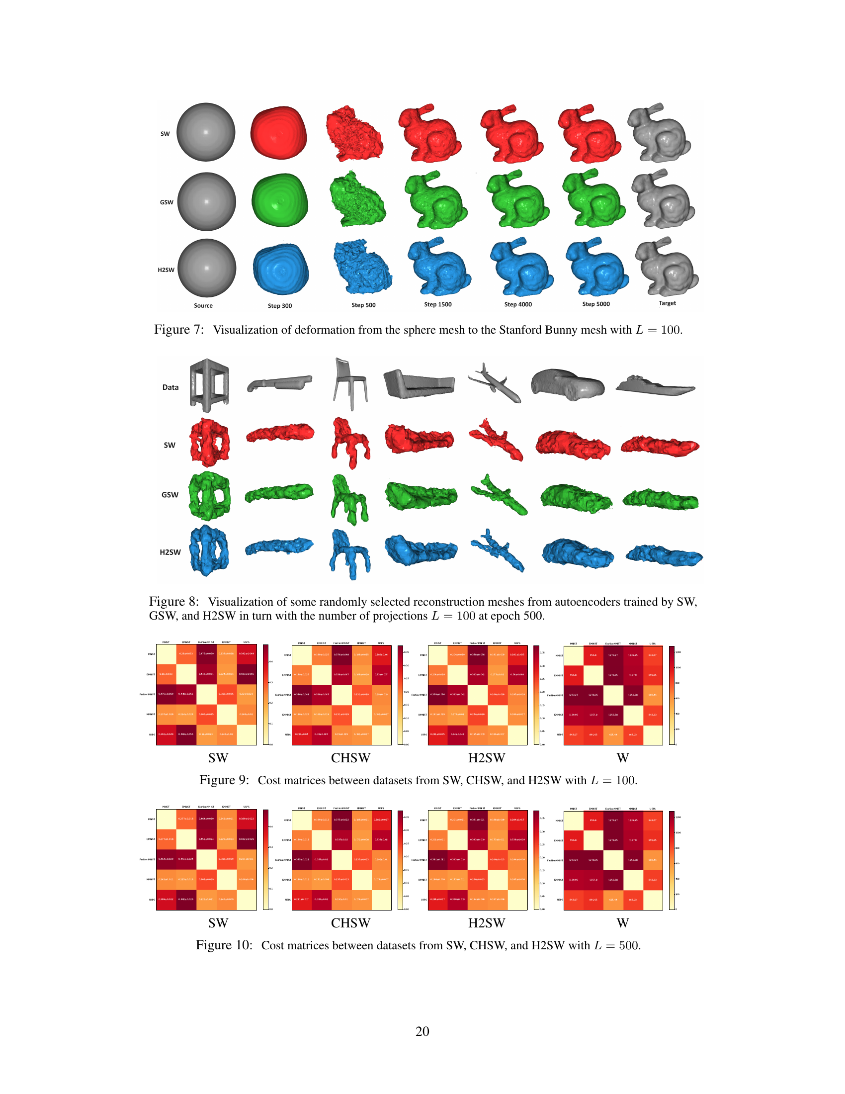
This figure visualizes the deformation process from a sphere mesh to a Stanford Bunny mesh using three different Wasserstein distance methods: SW, GSW, and H2SW. Each row represents a different method, showing the intermediate steps of the deformation at various time points (Step 300, Step 500, Step 1500, Step 4000, Step 5000). The number of projections (L) used in the calculation is 100. The figure demonstrates the visual differences in the deformation process produced by each method, highlighting the different ways they capture and represent the transformation between shapes. The target mesh is shown on the far right.
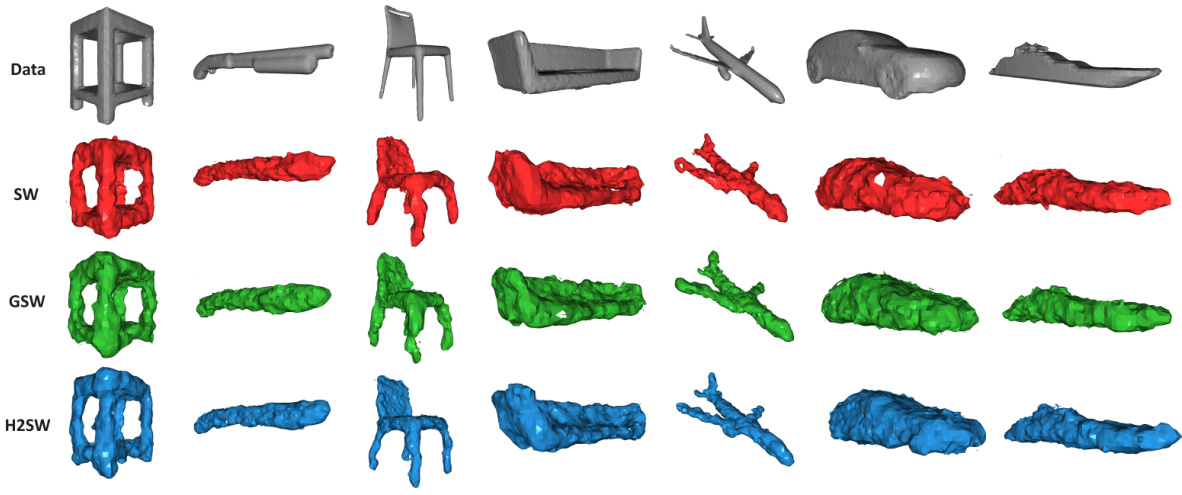
This figure shows the 3D reconstruction results of randomly selected meshes from the trained autoencoders using SW, GSW, and H2SW methods. The number of projections (L) used was 100, and the models were evaluated at epoch 500 of the training process. The image provides a visual comparison of the reconstruction quality achieved by each method.

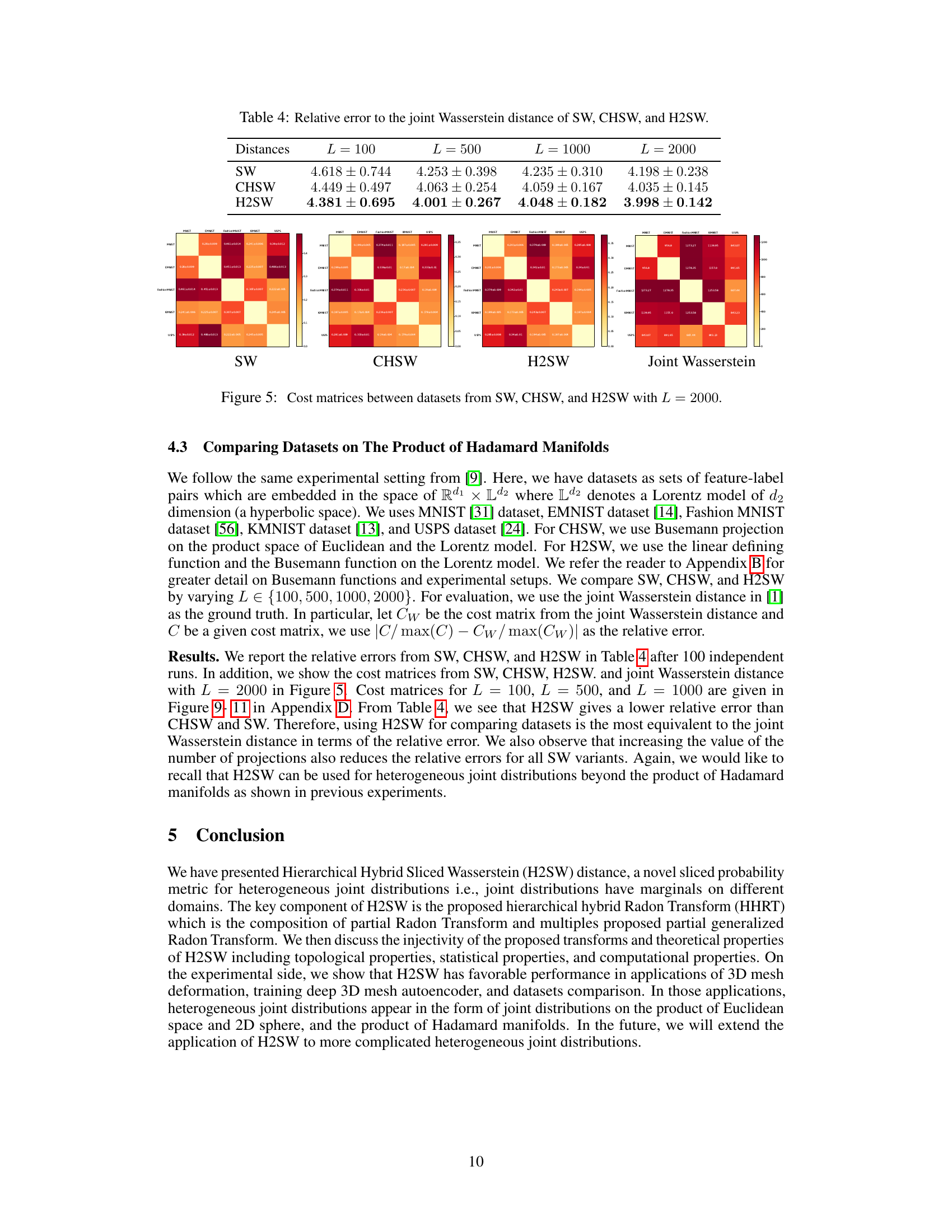
This figure shows the cost matrices obtained using three different methods: Sliced Wasserstein (SW), Cartan-Hadamard Sliced Wasserstein (CHSW), and Hierarchical Hybrid Sliced Wasserstein (H2SW). Each matrix represents the pairwise distances between five different datasets (MNIST, EMNIST, Fashion MNIST, KMNIST, and USPS). The number of projections L is set to 2000. The color intensity represents the magnitude of the distance, with darker colors indicating larger distances and lighter colors indicating smaller distances. The figure helps to visually compare the similarities and differences in the distance calculations between the three methods, highlighting how H2SW’s results compare to the ground truth (Joint Wasserstein) more closely than SW and CHSW.
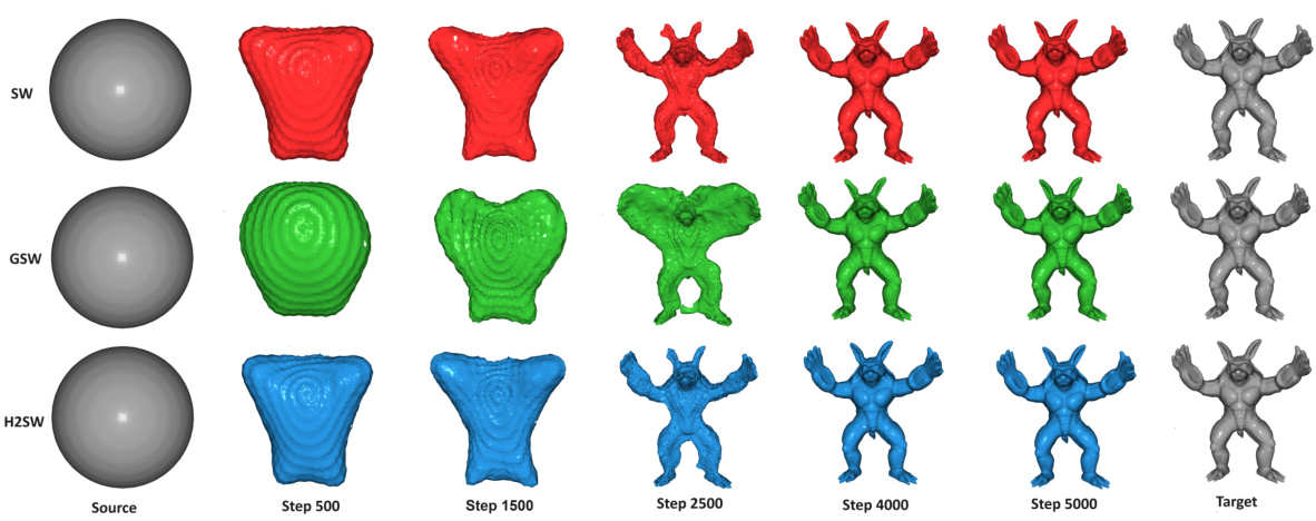
This figure visualizes the deformation process from a sphere mesh to an Armadillo mesh using three different Wasserstein distance methods: SW, GSW, and H2SW. Each row represents a different method, showing the intermediate steps of the deformation process at various time points (Step 500, 1500, 2500, 4000, and 5000) towards the final target Armadillo mesh. The parameter L, which refers to the number of projections, is set to 10 for this visualization. The differences in the intermediate steps and the final results highlight the distinct characteristics and effectiveness of the three methods in 3D mesh deformation.
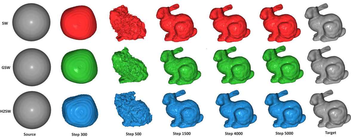
This figure shows a sequence of 3D mesh deformations from a sphere to a Stanford Bunny model using three different sliced Wasserstein distances: SW (top row), GSW (middle row), and H2SW (bottom row). Each row displays the source mesh (leftmost), intermediate steps of the deformation at steps 300, 500, 1500, 4000, and 5000, and the target mesh (rightmost). The number of projections (L) used in all methods is 100. The purpose of the figure is to visually compare the results obtained by each method, highlighting the differences in the progression of the deformation and the final result.

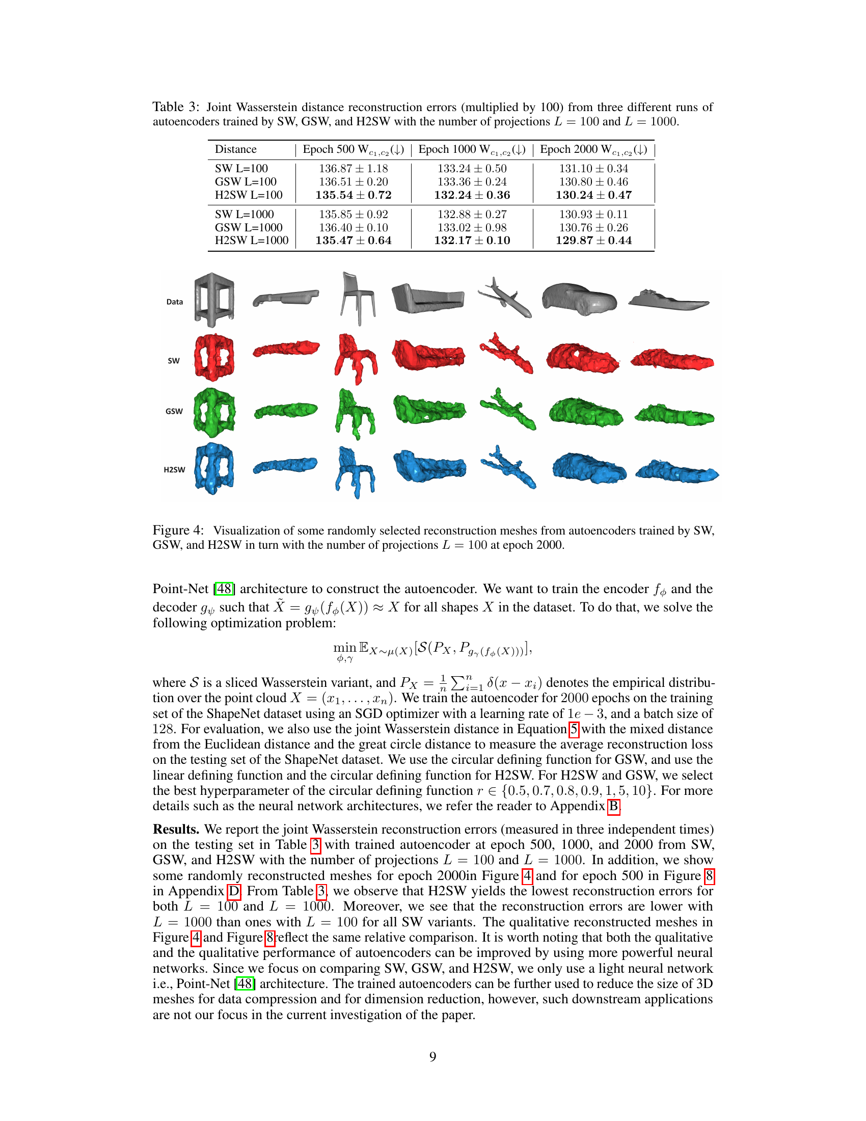
This figure visualizes the reconstruction results from autoencoders trained using three different sliced Wasserstein distances: SW, GSW, and the proposed H2SW. Each column represents a different input 3D mesh from the ShapeNet dataset. The rows show the reconstructions generated by each of the three methods. The number of projections L was set to 100, and the results are shown at epoch 2000 of training. The figure allows for a qualitative comparison of the reconstruction quality produced by each method.

This figure displays a comparison of cost matrices generated using three different methods: Sliced Wasserstein (SW), Cartan-Hadamard Sliced Wasserstein (CHSW), and Hierarchical Hybrid Sliced Wasserstein (H2SW). Each matrix shows the pairwise distances between five different datasets: MNIST, EMNIST, Fashion MNIST, KMNIST, and USPS. The matrices are visualized as heatmaps, with warmer colors indicating larger distances. The purpose is to illustrate the relative accuracy of H2SW compared to other methods in reflecting the true joint Wasserstein distance between the datasets.

This figure illustrates the Generalized Radon Transform (GRT) and the proposed Hierarchical Hybrid Radon Transform (HHRT) applied to a discrete distribution. It shows how GRT projects a high-dimensional distribution into a one-dimensional space, whereas HHRT, designed for heterogeneous joint distributions, first applies a partial GRT to each marginal component and then a partial Radon Transform (PRT) on the joint transformed arguments, to integrate marginal information. The diagram visually represents the steps of each transform, highlighting the different operations and outputs.

This figure displays cost matrices generated using three different methods: Sliced Wasserstein (SW), Cartan-Hadamard Sliced Wasserstein (CHSW), and Hierarchical Hybrid Sliced Wasserstein (H2SW), with the number of projections L set to 2000. Each matrix visualizes the pairwise distances between five datasets: MNIST, EMNIST, Fashion MNIST, KMNIST, and USPS. The color intensity represents the distance, with darker colors indicating greater distances and lighter colors indicating smaller distances. The figure visually compares the results of these three methods against the Joint Wasserstein distance, providing a qualitative comparison of their effectiveness in measuring the similarity between datasets.
More on tables

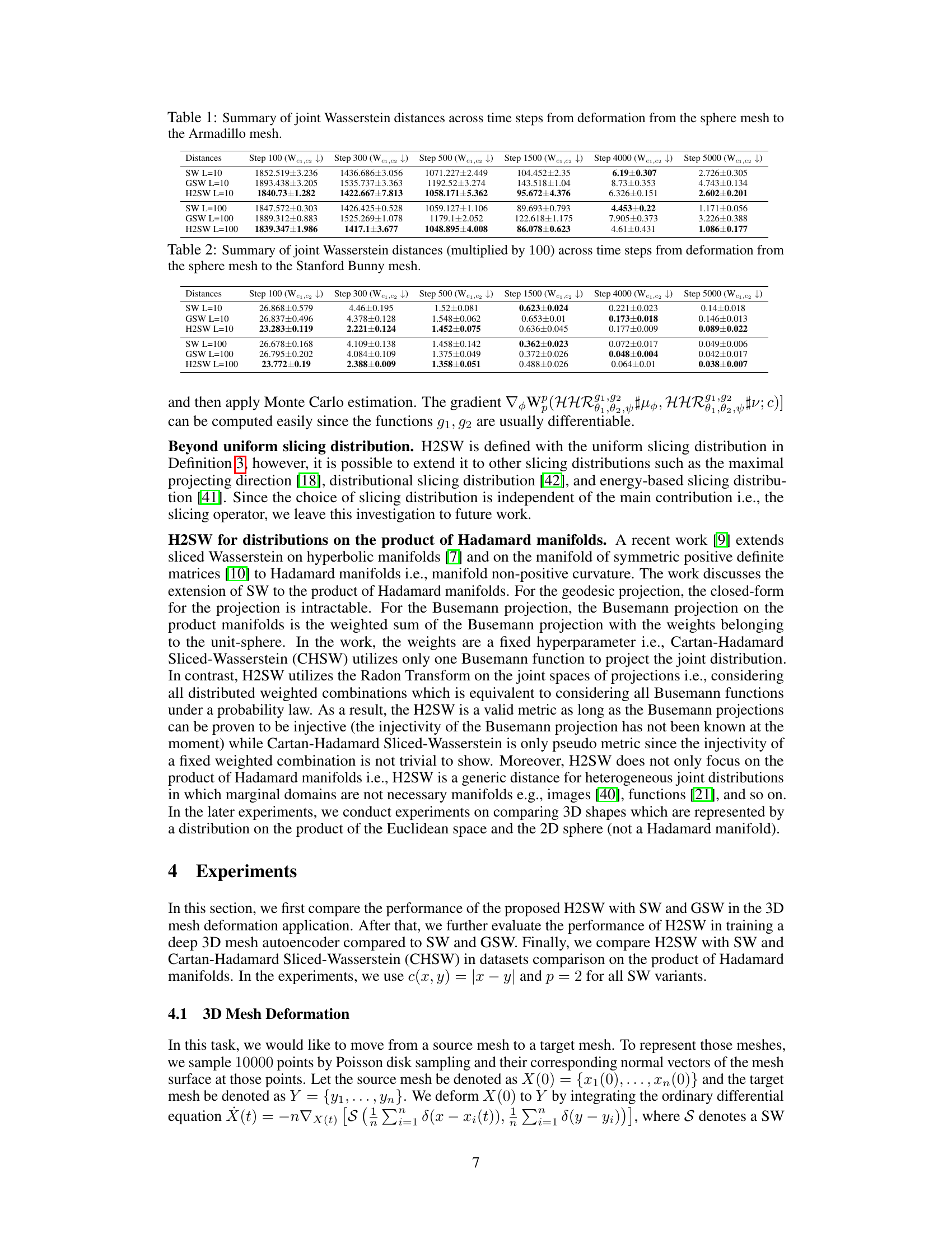
This table presents the quantitative results of comparing three different sliced Wasserstein variants (SW, GSW, and H2SW) in a 3D mesh deformation task. The experiment deforms a sphere mesh into a Stanford Bunny mesh using an optimization process and measures the distance between the deformed mesh and the target mesh at various steps. The table shows the joint Wasserstein distance for each method using different numbers of projections (L=10 and L=100). Lower distances indicate better performance.

This table presents the joint Wasserstein distance reconstruction errors for autoencoders trained using three different sliced Wasserstein variants (SW, GSW, and H2SW). The errors are shown for three independent runs at epochs 500, 1000, and 2000, with two different numbers of projections (L=100 and L=1000). Lower values indicate better performance.

This table presents the relative errors of three different methods (SW, CHSW, and H2SW) compared to the joint Wasserstein distance. The relative error is calculated as the absolute difference between the normalized cost matrices of each method and the normalized joint Wasserstein cost matrix. The results are shown for four different numbers of projections (L): 100, 500, 1000, and 2000. Lower relative errors indicate better approximations to the ground truth (joint Wasserstein distance).
Full paper#
