↗ OpenReview ↗ NeurIPS Homepage ↗ Chat
TL;DR#
Reconstructing accurate 3D surfaces from point cloud data is a challenging task in computer vision. Existing neural network-based methods often struggle to capture fine details and tend to smooth out local features, limiting the accuracy of the final reconstruction. This is mainly due to the lack of ground truth data or ambiguities in estimating SDFs directly from raw point clouds.
MultiPull tackles this challenge by introducing a novel framework that learns multi-scale implicit fields from raw point clouds. It progressively pulls multi-level query points onto the surface via a multi-step optimization process. This approach leverages the power of frequency features to capture geometry at different levels of detail. Furthermore, by incorporating spatial distance and normal consistency constraints during optimization, the method significantly improves the accuracy of the SDF estimates and achieves superior performance in 3D surface reconstruction compared to state-of-the-art techniques. The effectiveness is demonstrated through experiments on widely-used benchmarks.
Key Takeaways#
Why does it matter?#
This paper is important because it presents a novel method for reconstructing 3D surfaces from point clouds, addressing the limitations of existing methods by using multi-scale features and optimization strategies. This significantly improves the accuracy and detail of 3D surface reconstruction, which has broad applications in computer vision and related fields. The method’s effectiveness on various benchmarks demonstrates its potential impact on numerous applications, and it opens new avenues for research in implicit surface representation and multi-scale optimization.
Visual Insights#
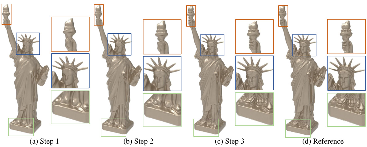
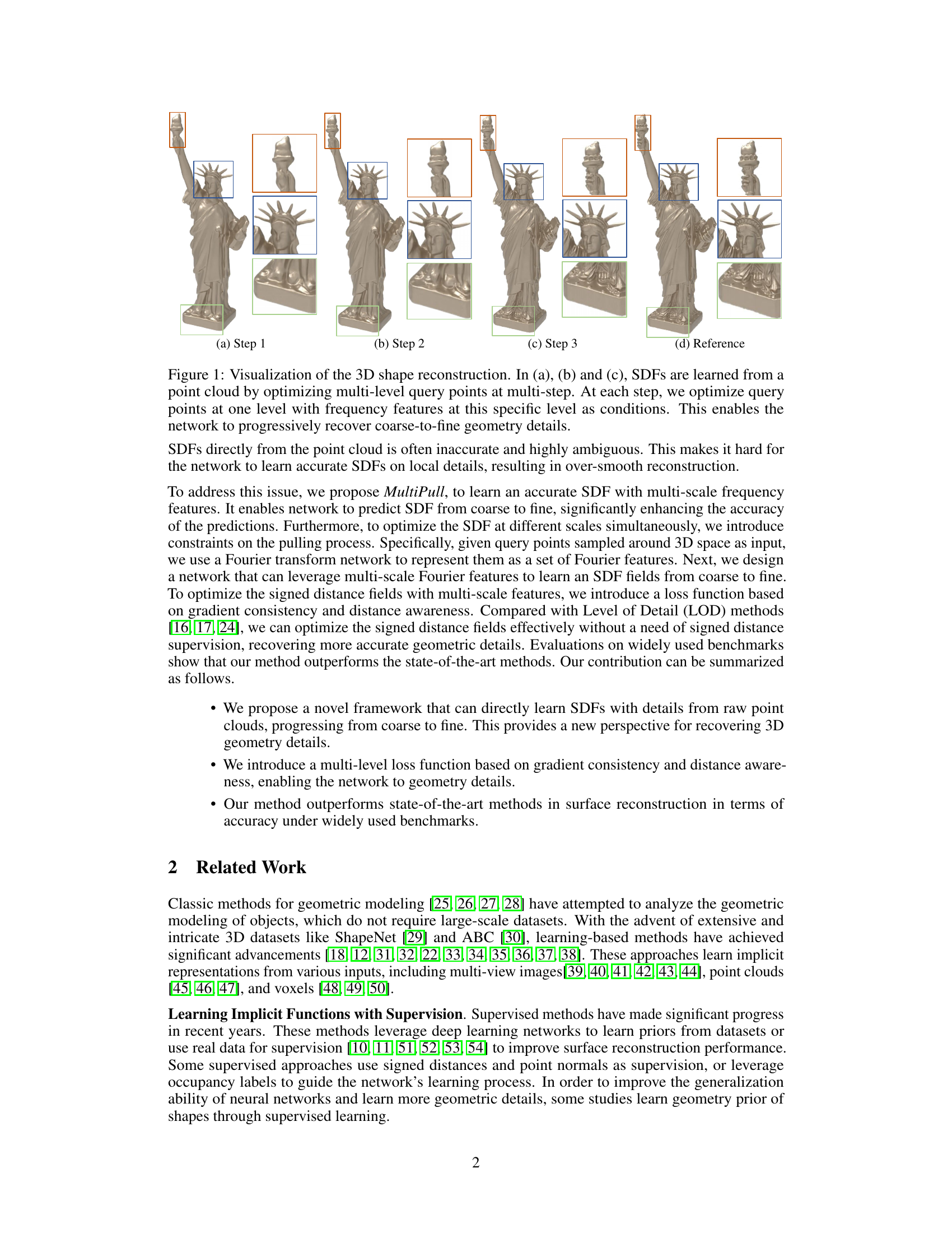
This figure shows the process of 3D shape reconstruction using the MultiPull method. The reconstruction is shown in three steps, with each step refining the detail from a coarse to fine level. The final reconstruction is compared to the ground truth model. Multi-level query points and frequency features are used to achieve accurate SDF learning.

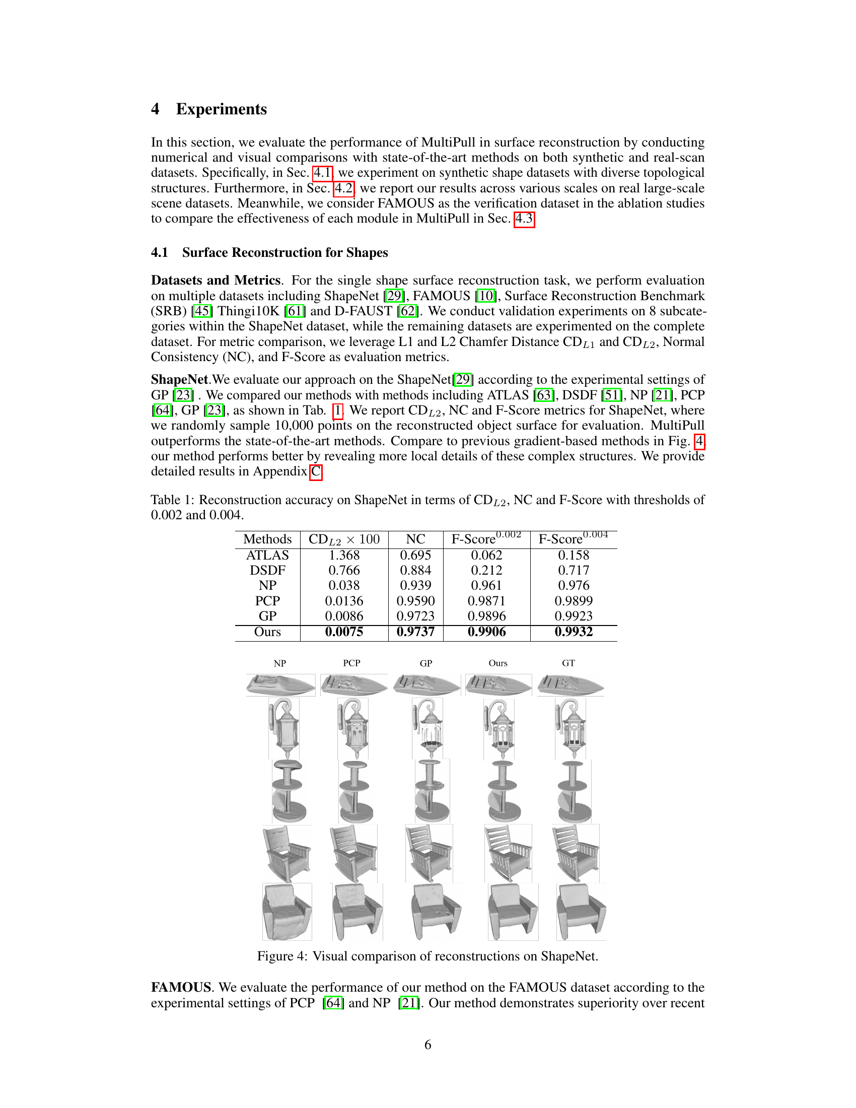
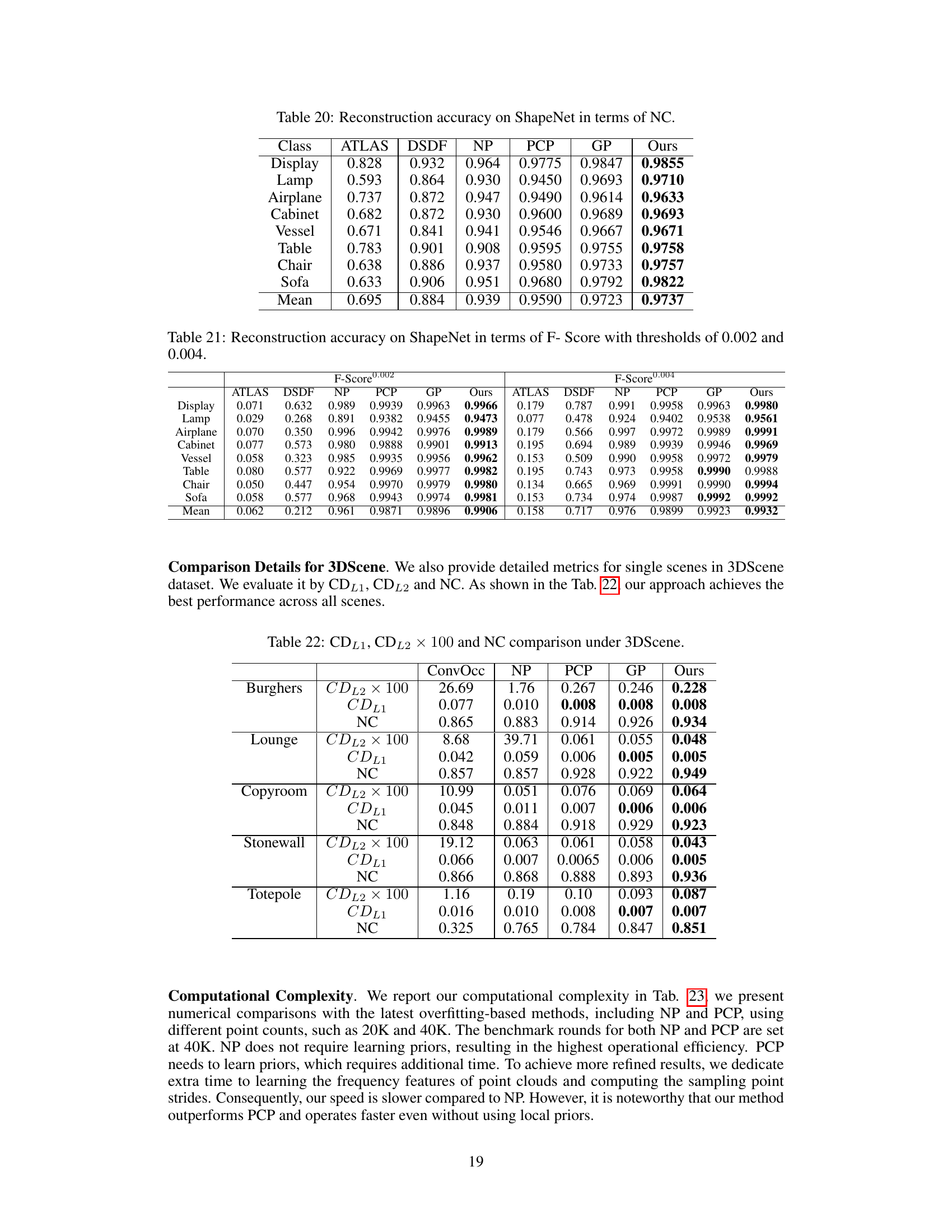
This table presents a comparison of the performance of different methods for surface reconstruction on the ShapeNet dataset. The metrics used are Chamfer Distance (CDL2), Normal Consistency (NC), and F-Score, which are calculated at two different thresholds (0.002 and 0.004). The methods compared include ATLAS, DSDF, NP, PCP, GP, and the authors’ proposed method, MultiPull. The table shows that MultiPull achieves the highest accuracy across all metrics and thresholds.
In-depth insights#
Multi-Scale SDFs#
Multi-scale SDFs represent a powerful approach to 3D shape reconstruction by representing the surface at multiple levels of detail simultaneously. Lower resolutions capture the overall shape and coarser features, while higher resolutions refine finer details and intricate geometries. This approach addresses limitations of single-scale methods that often struggle to balance overall shape accuracy with fine-grained detail. By using a hierarchy of SDFs, the computational cost can be managed more efficiently, as coarse levels can be computed quickly, while high-resolution details are only focused on in specific regions of interest. This leads to more robust and efficient 3D shape representation. Moreover, multi-scale SDFs often incorporate techniques such as frequency features or level-of-detail (LOD) strategies to further optimize the learning process and achieve higher-quality reconstructions. The ability to progressively refine a shape from coarse to fine enables handling of large point clouds more effectively and efficiently, and leads to a more comprehensive understanding and modeling of the underlying surface geometry.
Multi-Step Pulling#
The concept of “Multi-Step Pulling” in the context of 3D surface reconstruction from point clouds suggests an iterative refinement process. It likely involves repeatedly adjusting query points’ positions, pulling them towards the estimated surface at each step. This iterative approach likely improves accuracy by progressively resolving ambiguities and refining the surface representation. Each step refines the previous estimate, leveraging updated information from the point cloud and the evolving implicit function. The multi-step aspect is crucial for handling noise and the inherent sparsity of point cloud data, allowing the algorithm to gradually converge to a more accurate and detailed reconstruction. The strategy likely incorporates feedback loops and potentially utilizes gradient information at each step to guide the refinement process towards the actual surface. It’s a clever way to avoid pitfalls of single-step methods and achieve finer detail.
Frequency Features#
The concept of “Frequency Features” in this context likely refers to a method of representing data points from a 3D point cloud in a way that captures different levels of detail or frequency of geometric information. Instead of directly using the raw spatial coordinates, the method transforms these coordinates into a frequency domain representation, possibly utilizing techniques like the Fourier transform. This allows the model to learn multi-scale features more effectively. Lower frequencies would capture the overall shape and larger-scale structures, while higher frequencies would represent finer details and local geometry. This multi-scale approach is key to overcoming challenges related to over-smoothing in traditional methods that tend to lose fine geometric details. By separating the information into different frequency bands, the model can learn and optimize the signed distance function (SDF) at multiple scales simultaneously. This hierarchical approach enables a progressive refinement from coarse to fine, resulting in a more accurate and detailed 3D surface reconstruction.
Loss Function Design#
The effectiveness of any deep learning model hinges significantly on the design of its loss function. A well-crafted loss function guides the model’s learning process towards achieving the desired outcome, in this case, accurate surface reconstruction from point clouds. The authors likely explored several options, potentially starting with standard geometric loss functions like Chamfer distance or Earth Mover’s distance, which measure the discrepancy between the predicted surface and the ground truth point cloud. However, limitations of these basic approaches, such as sensitivity to outliers and inability to capture fine-grained details, would likely motivate the exploration of more advanced loss functions. Multi-level loss functions could address this by incorporating constraints at various levels of detail, ensuring both global consistency and accurate local features are captured. Moreover, incorporating normal consistency within the loss function is crucial for smooth surface reconstruction; it would penalize inconsistencies in surface normals between neighboring points, leading to a more coherent and realistic surface. The authors might have combined several loss terms, each addressing a specific aspect of the problem. This approach allows for a more fine-tuned optimization and a more balanced model, ensuring accurate SDF predictions across different scales and preventing over-smoothing or the introduction of artifacts. The weighting of individual loss components is another critical aspect, requiring careful tuning for optimal performance. Therefore, a robust loss function design, likely a multi-component loss with carefully balanced weights and appropriate regularization, was fundamental for achieving the superior results reported by the authors.
Future Directions#
Future research could explore several promising avenues. Improving the efficiency and scalability of the MultiPull framework is crucial, perhaps through exploring more efficient multi-level representations and optimization strategies. Addressing the challenges posed by noisy or incomplete point clouds remains a key area; incorporating robust methods for outlier detection and noise reduction would significantly improve the accuracy and reliability of surface reconstruction. Expanding the application domain to handle larger and more complex scenes, such as those encountered in autonomous driving and robotics, would be a significant advancement. Investigating the potential of incorporating additional sensor modalities, such as RGB images and depth maps, to enhance the quality of reconstructed surfaces could significantly improve the realism and detail of the results. Finally, developing a more thorough theoretical understanding of the underlying principles of MultiPull and its relationship to other implicit surface reconstruction methods will enable the development of even more sophisticated and effective approaches in the future.
More visual insights#
More on figures

This figure shows the architecture of the MultiPull method, which consists of two main modules: the Frequency Feature Transformation (FFT) module and the Multi-Step Pulling (MSP) module. The FFT module transforms query points into multi-level frequency features, while the MSP module uses these features to iteratively refine the SDF predictions, progressively recovering more detailed geometry information.
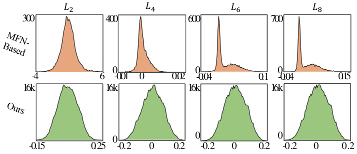
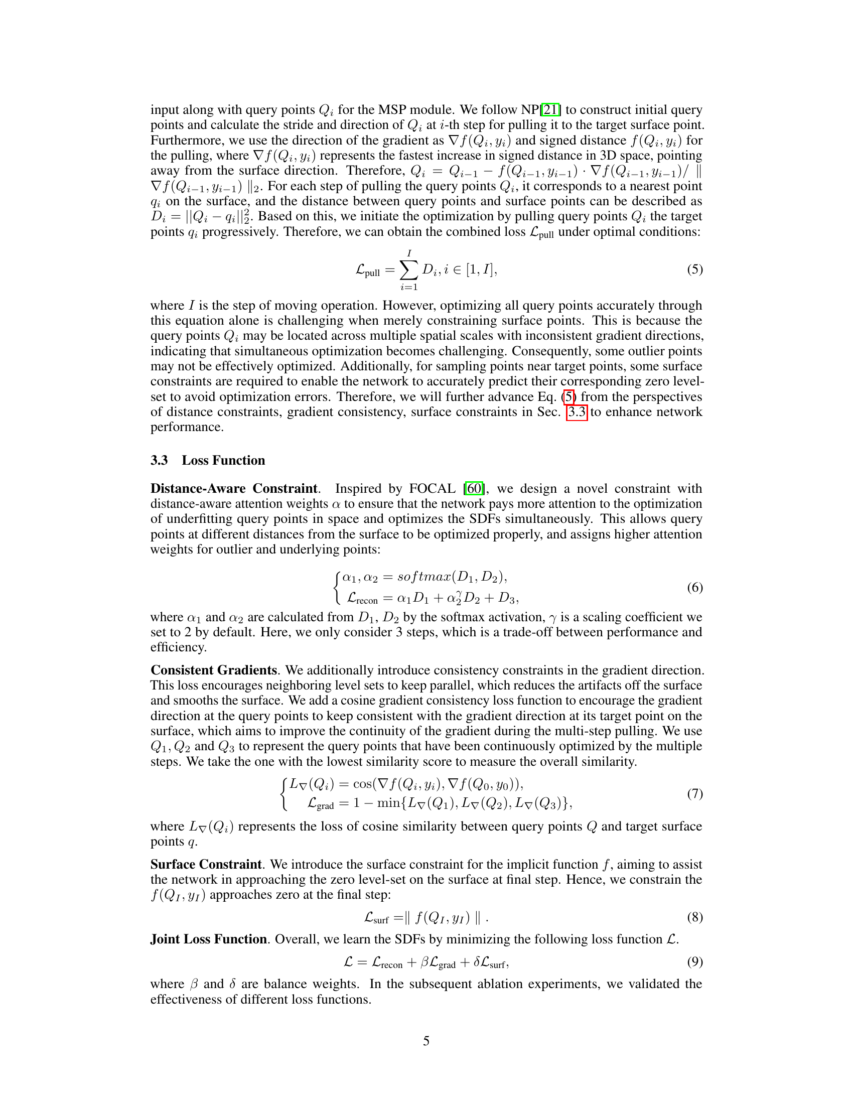
This figure compares the parameter distributions of different linear layers (L2, L4, L6, L8) using two different initialization methods: MFN-based and the proposed method. The MFN-based method shows gradient vanishing and small activations in deeper layers, while the proposed method ensures that the parameters of each linear layer follow a standard normal distribution, leading to improved performance in the reconstruction task. The Appendix B provides further visual details on these effects.
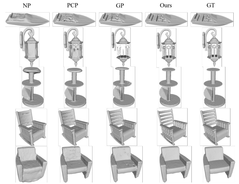
This figure shows a visual comparison of 3D shape reconstruction results on the ShapeNet dataset. It compares the results from four different methods: NP, PCP, GP, and the authors’ proposed MultiPull method, alongside the ground truth (GT). Each row displays the reconstruction of a different object from the dataset using the five different methods. The images visually demonstrate that the MultiPull method produces results that are closest to the ground truth in terms of both overall shape and fine details.

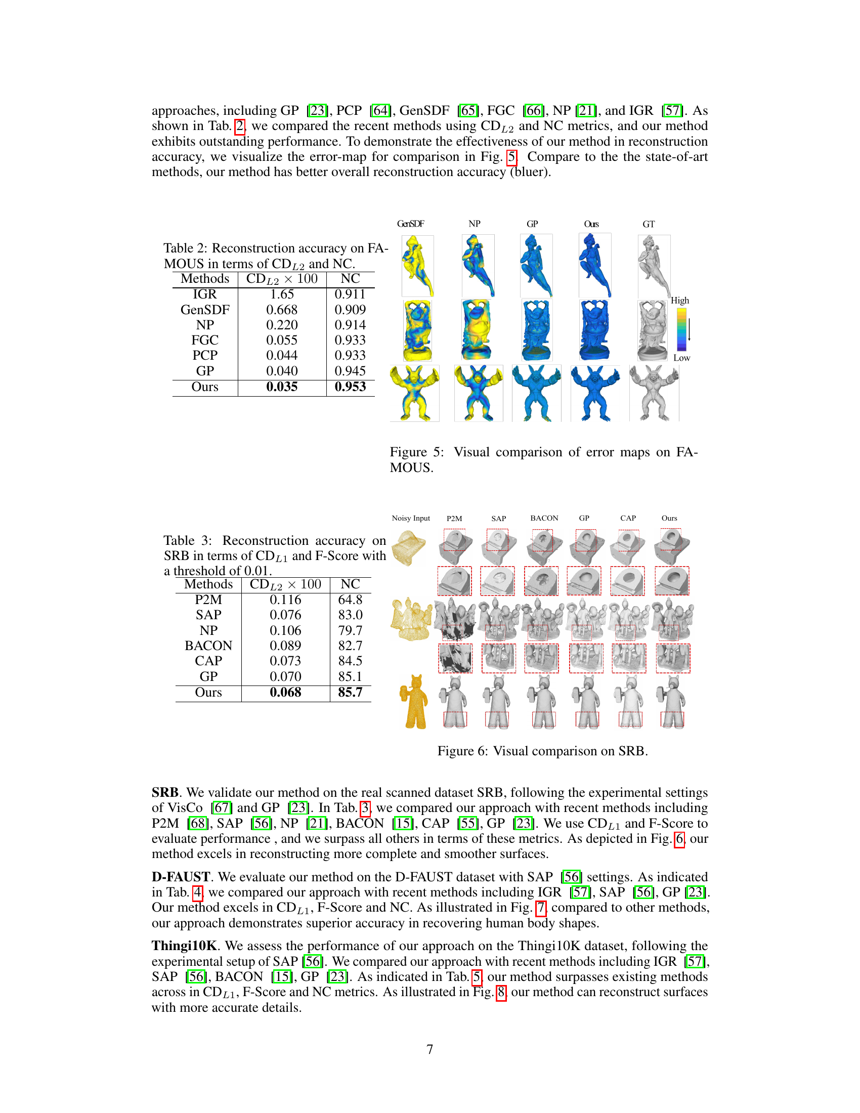
This figure displays a visual comparison of 3D shape reconstructions generated by several different methods (GenSDF, NP, PCP, GP, and the proposed MultiPull method) on the ShapeNet dataset. Each row shows the reconstruction of a different object, with the ground truth (GT) model shown in the rightmost column. The color maps on the reconstructed models indicate the error level, with blue representing lower errors and yellow/red indicating higher errors. The figure visually demonstrates the superiority of the MultiPull method in terms of accuracy and detail preservation in the reconstructions.
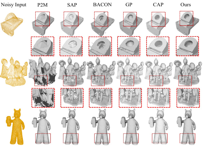
This figure compares the 3D surface reconstruction results from different methods on the SRB dataset. The first column shows the noisy input point clouds. Subsequent columns display reconstruction results from P2M, SAP, BACON, GP, CAP, and the proposed MultiPull method. Red boxes highlight areas where MultiPull demonstrates superior performance in detail preservation and noise handling. The comparison highlights MultiPull’s ability to capture finer details and achieve more complete and smoother surface reconstructions.
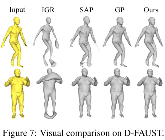
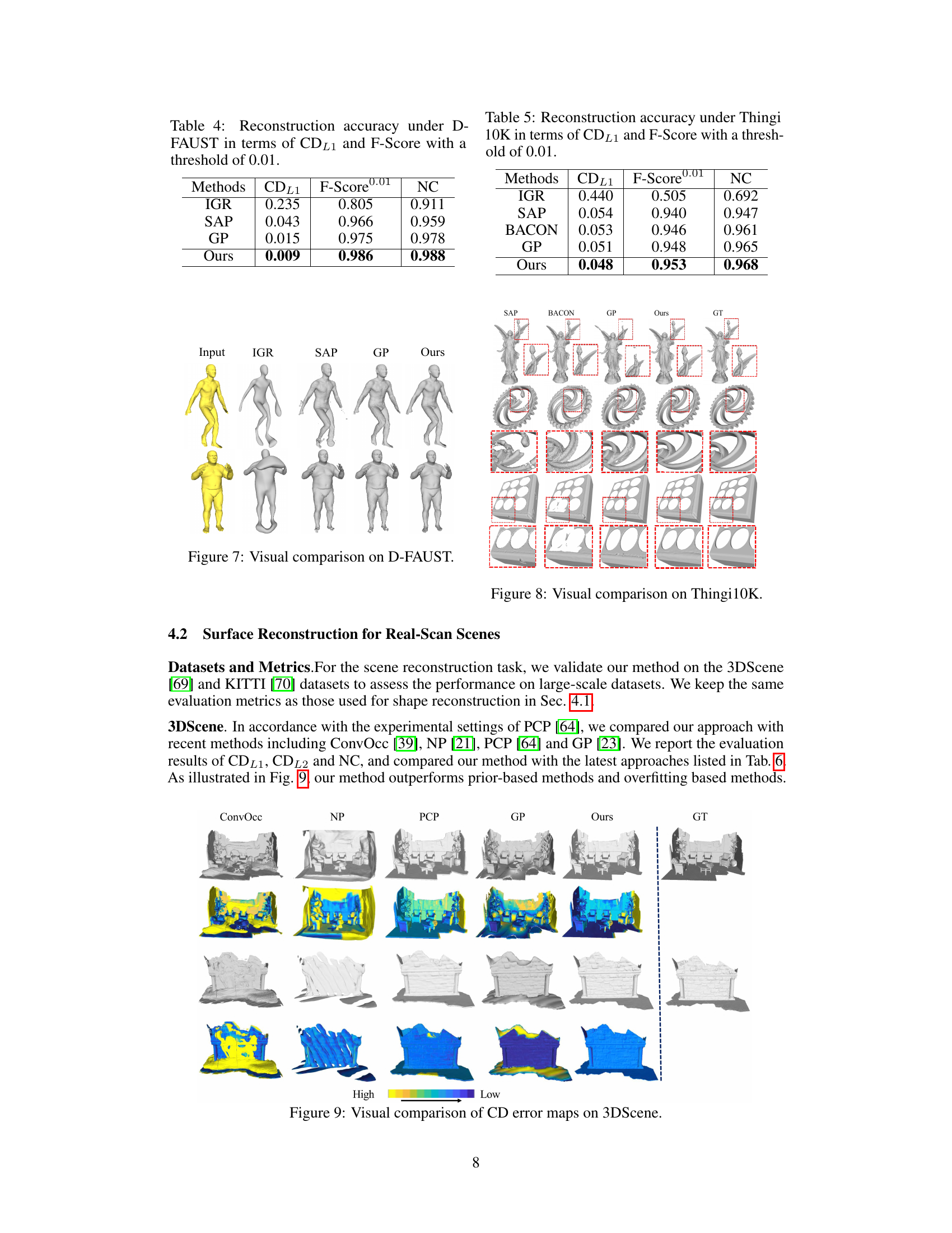
This figure compares the 3D reconstruction results of the proposed MultiPull method against three state-of-the-art methods (IGR, SAP, GP) on the D-FAUST dataset. The input is a point cloud representation of a human figure. The figure visually demonstrates MultiPull’s superior ability to reconstruct fine details and complete shapes, compared to the other methods, which exhibit artifacts or incompleteness in their reconstructions.
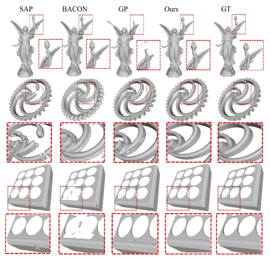
This figure presents a visual comparison of 3D shape reconstructions generated by different methods on the ShapeNet dataset. The top row shows the reconstruction of a statue; the second row displays a gear; the third and fourth rows show more complex objects. Each column represents a different reconstruction method: SAP, BACON, GP, the proposed MultiPull method, and the ground truth (GT). The red boxes highlight areas where the proposed method demonstrates improved detail and accuracy compared to other approaches.
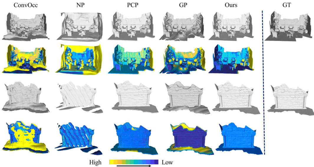
This figure shows a visual comparison of the reconstruction results on the 3DScene dataset for different methods including ConvOcc, NP, PCP, GP, and the proposed MultiPull method. The CD error maps are visualized, showing the error distribution across the reconstructed surfaces. Lower CD error values (shown in blue) indicate better reconstruction accuracy. MultiPull demonstrates improved reconstruction performance with lower errors compared to the other methods.
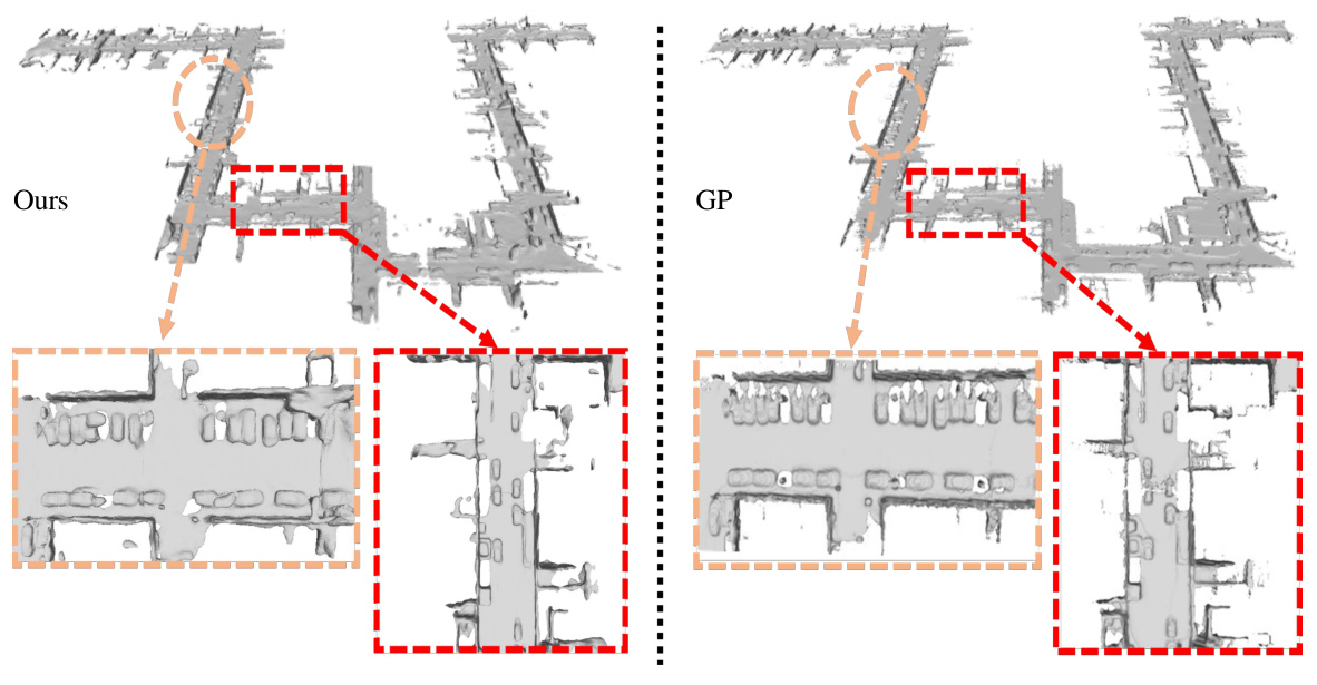
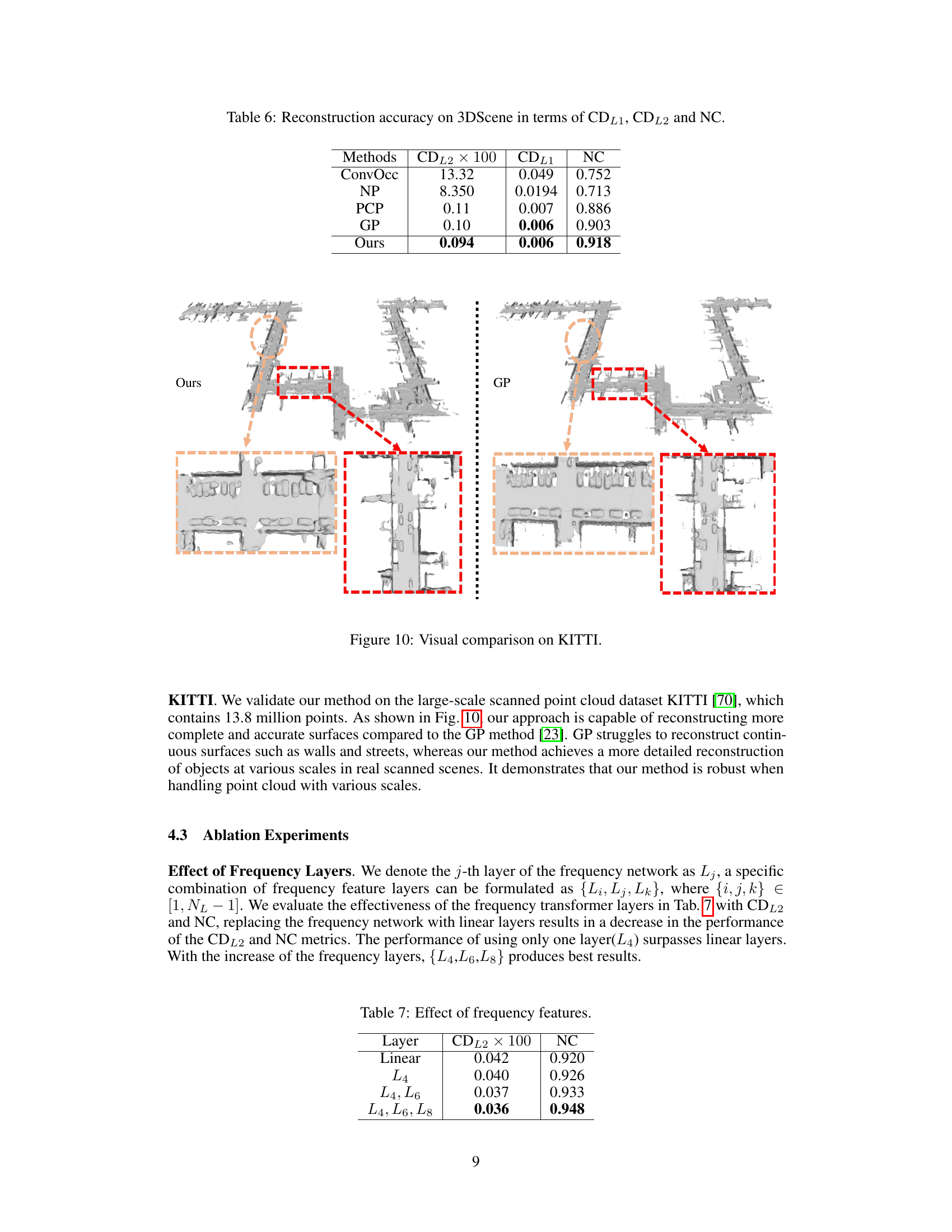
This figure compares the surface reconstruction results of the proposed MultiPull method and the GP method on the KITTI dataset. The left image shows the reconstruction by MultiPull, and the right image shows the reconstruction by GP. Both images show a portion of a scene which contains walls and a corridor. The dashed red lines highlight some regions to better illustrate the differences in the results. MultiPull produces a more complete reconstruction, especially around the walls, demonstrating its superior performance in reconstructing large-scale scenes.
The figure compares the parameter distributions of different linear layers (L2, L4, L6, L8) using two different initialization methods: MFN-based and the proposed method. The MFN-based method shows gradient vanishing and small activations in deeper layers, while the proposed method ensures parameters follow a standard normal distribution for each linear layer. This visualization is supplemented by Appendix B, which likely contains further results demonstrating the positive effects of the proposed method on reconstruction.
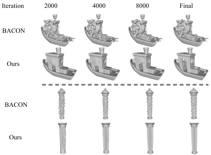
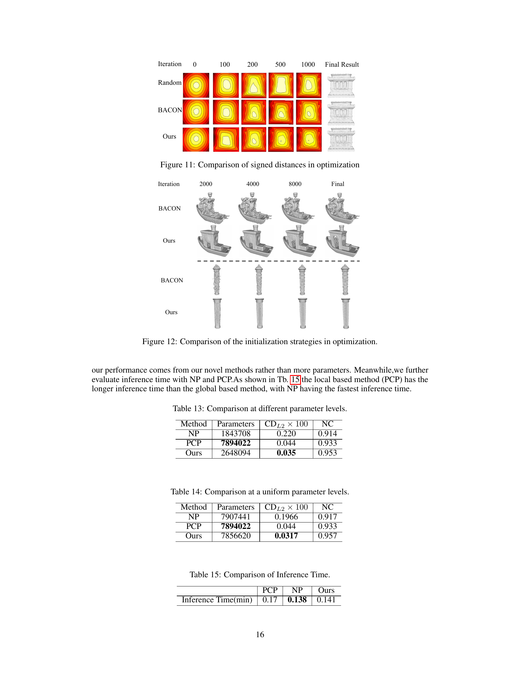
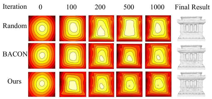
This figure compares the optimization process of signed distance functions using different initialization strategies: random, BACON, and the proposed method. It shows the reconstruction results at different iterations (2000, 4000, 8000) and the final result for two different shapes: a boat and a column. The visualization demonstrates how the proposed method converges faster and produces more accurate reconstructions than the baselines, particularly BACON.
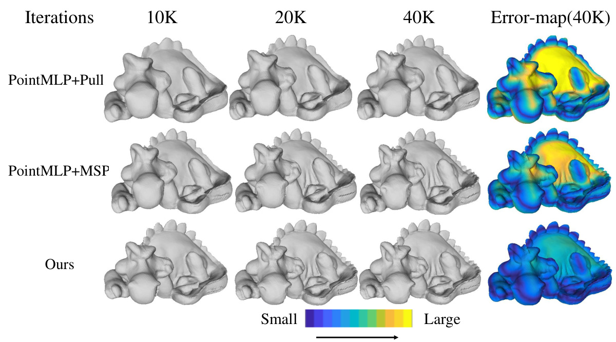
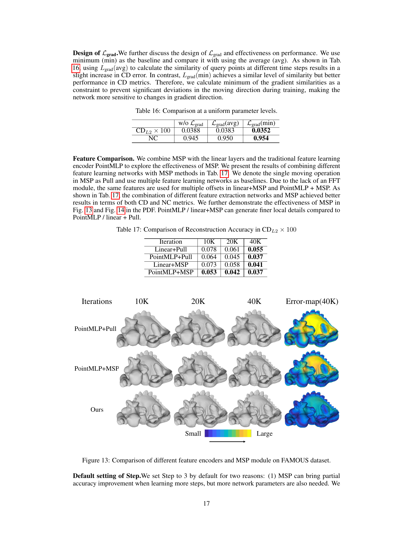
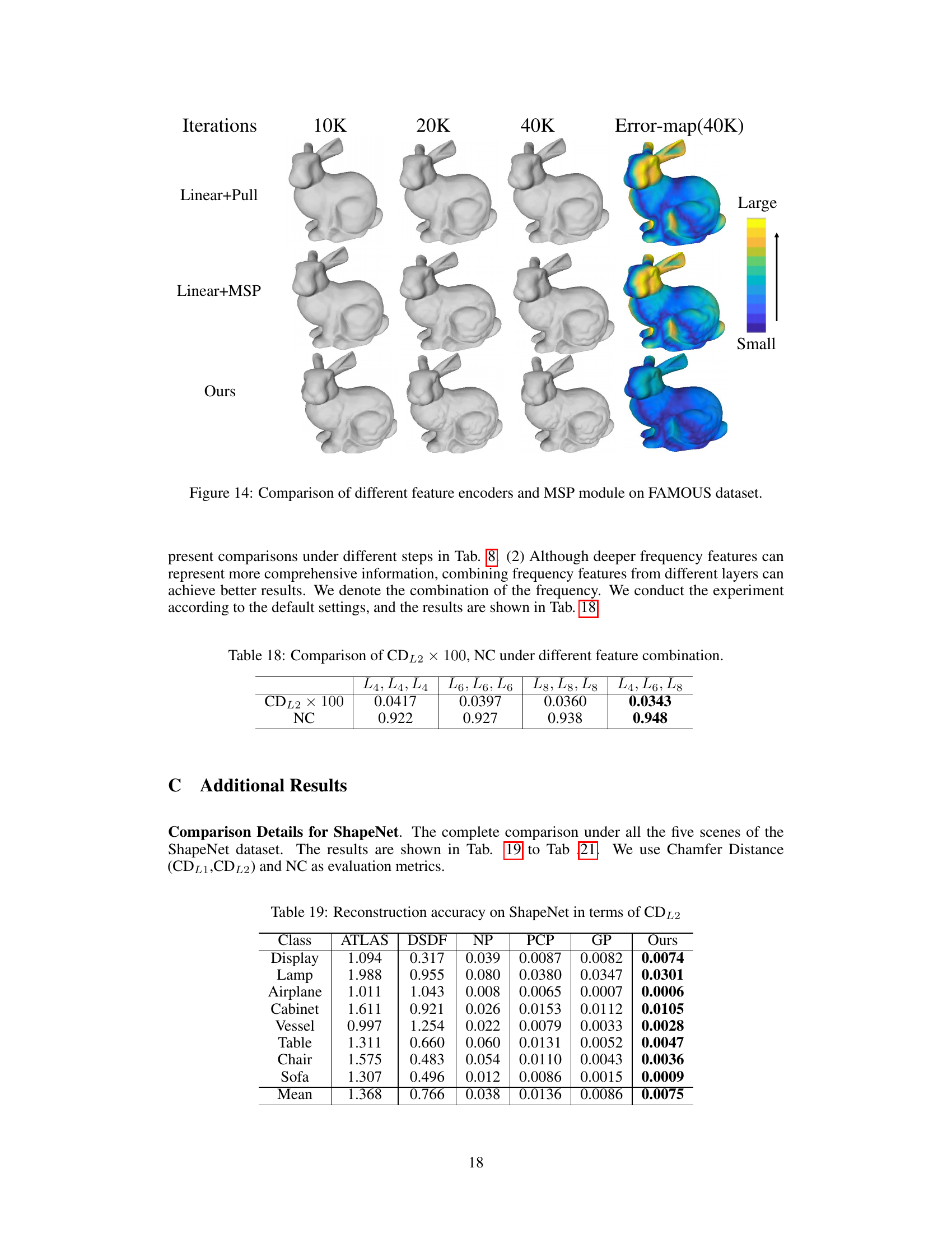
This figure compares the 3D shape reconstruction results obtained using different feature encoders (linear layers and PointMLP) combined with either the single-step pulling (Pull) or the multi-step pulling (MSP) module of the proposed MultiPull method. The comparison is shown for different numbers of training iterations (10K, 20K, and 40K). The error maps (40K) visualize the difference between the reconstructed surfaces and the ground truth, with color intensity representing the magnitude of the error. The results show that using MSP with either linear layers or PointMLP significantly improves the accuracy and detail of the reconstruction compared to using the single-step Pull method. The MultiPull method, which uses the FFT module and MSP, outperforms both other configurations.
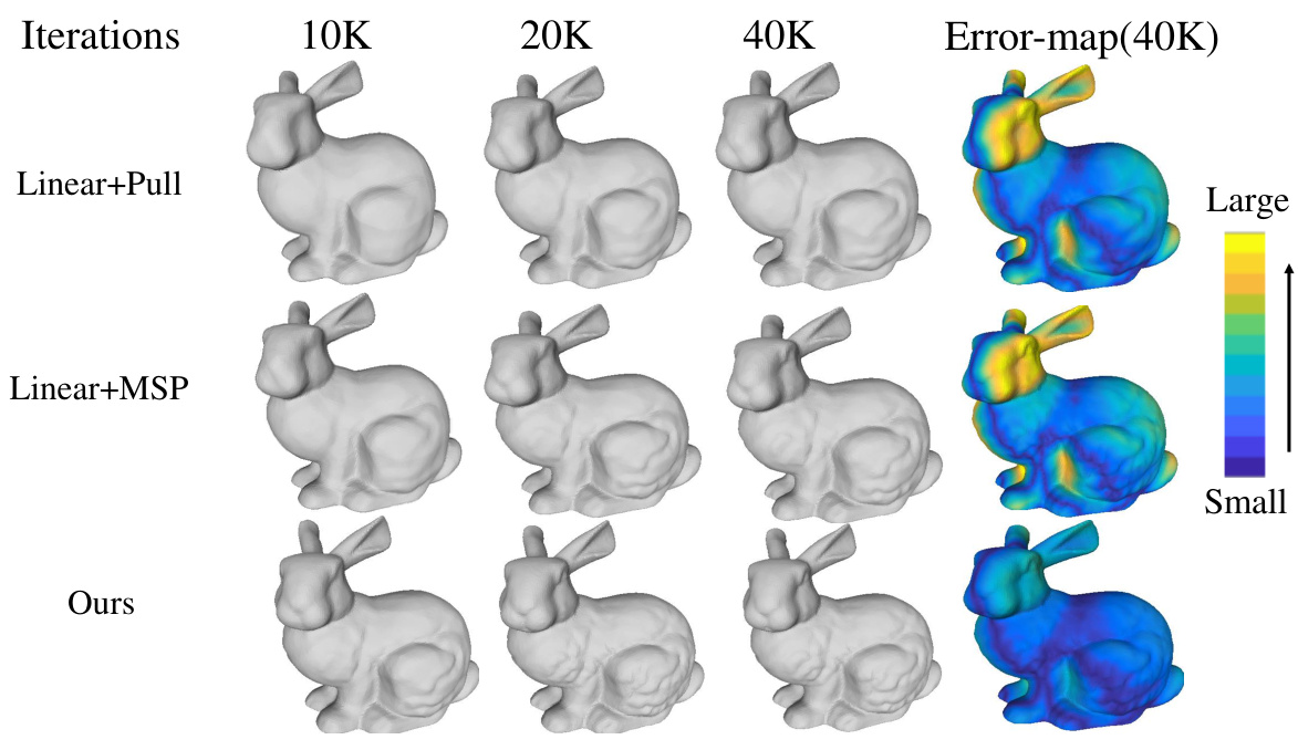
This figure shows a comparison of the reconstruction results using different feature encoders (linear and PointMLP) and the Multi-Step Pulling (MSP) module on the FAMOUS dataset. It visually demonstrates that combining MSP with either linear features or PointMLP features leads to more detailed and accurate reconstructions, particularly with 40k iterations, as indicated by the error maps (showing small errors in blue and larger errors in yellow/red). The figure highlights the effectiveness of the MSP module in enhancing the quality of 3D surface reconstruction.
More on tables
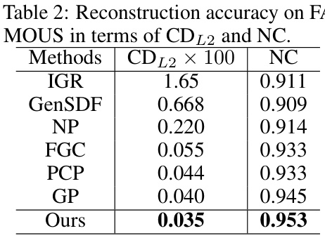
This table presents a comparison of the reconstruction accuracy achieved by different methods on the FAMOUS dataset. The accuracy is measured using two metrics: Chamfer Distance (CDL2) and Normal Consistency (NC). Lower values for CDL2 indicate better reconstruction accuracy, while higher values for NC indicate better normal consistency. The results show that the proposed ‘Ours’ method outperforms the state-of-the-art methods.

This table presents a comparison of the reconstruction accuracy achieved by different methods on the SRB dataset. The metrics used are the Chamfer Distance (CDL1) and F-Score, both calculated with a threshold of 0.01. The methods compared include P2M, SAP, NP, BACON, CAP, GP, and the authors’ proposed method, MultiPull. The results show that MultiPull outperforms the other methods, achieving the lowest CDL1 and highest F-Score.
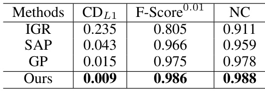
This table presents a comparison of the reconstruction accuracy achieved by different methods on the D-FAUST dataset. The metrics used for comparison are the Chamfer Distance (CDL1) and the F-Score, both calculated with a threshold of 0.01. The table highlights the superior performance of the proposed ‘Ours’ method compared to other state-of-the-art methods (IGR, SAP, GP).
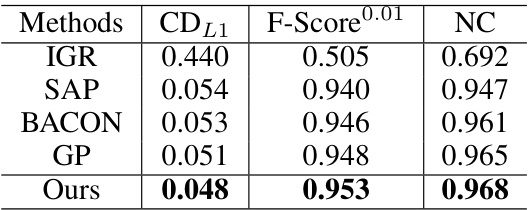
This table presents a quantitative evaluation of the MultiPull method’s performance on the D-FAUST dataset. The metrics used are the Chamfer Distance (CDL1), the F-Score (at a threshold of 0.01), and Normal Consistency (NC). The results are compared against several state-of-the-art methods (IGR, SAP, BACON, GP) to demonstrate the superior performance of MultiPull in terms of surface reconstruction accuracy.
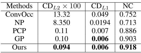
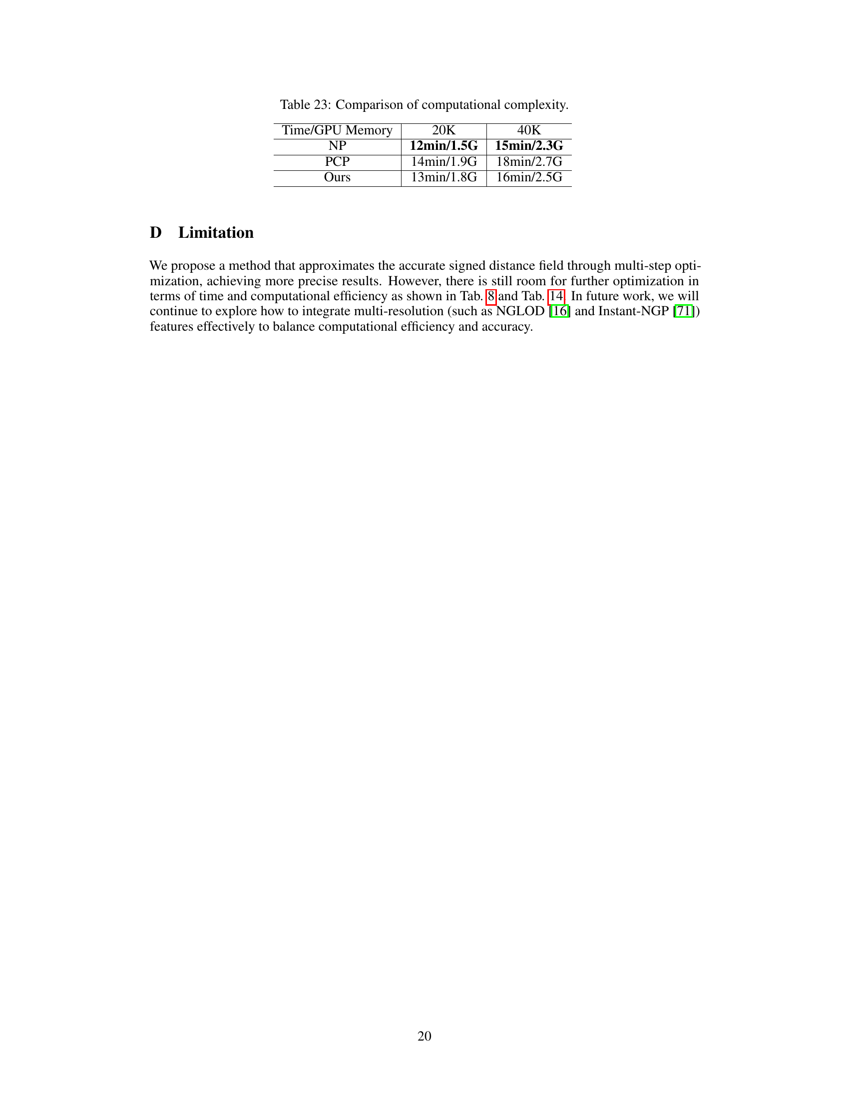
This table presents the quantitative results of surface reconstruction on the 3DScene dataset. It compares the performance of MultiPull against several state-of-the-art methods (ConvOcc, NP, PCP, GP) using three metrics: Chamfer Distance L1 (CDL1), Chamfer Distance L2 (CDL2), and Normal Consistency (NC). Lower values for CDL1 and CDL2 indicate better reconstruction accuracy, while a higher NC value signifies better normal alignment.
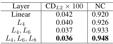
This table shows the effect of using different combinations of frequency layers (L4, L6, L8) in the Frequency Feature Transformation (FFT) module on the reconstruction accuracy, measured by CDL2 and NC. The results demonstrate that using multiple frequency layers, especially {L4, L6, L8}, improves the performance of the model compared to using only a single layer or linear layers.
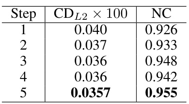
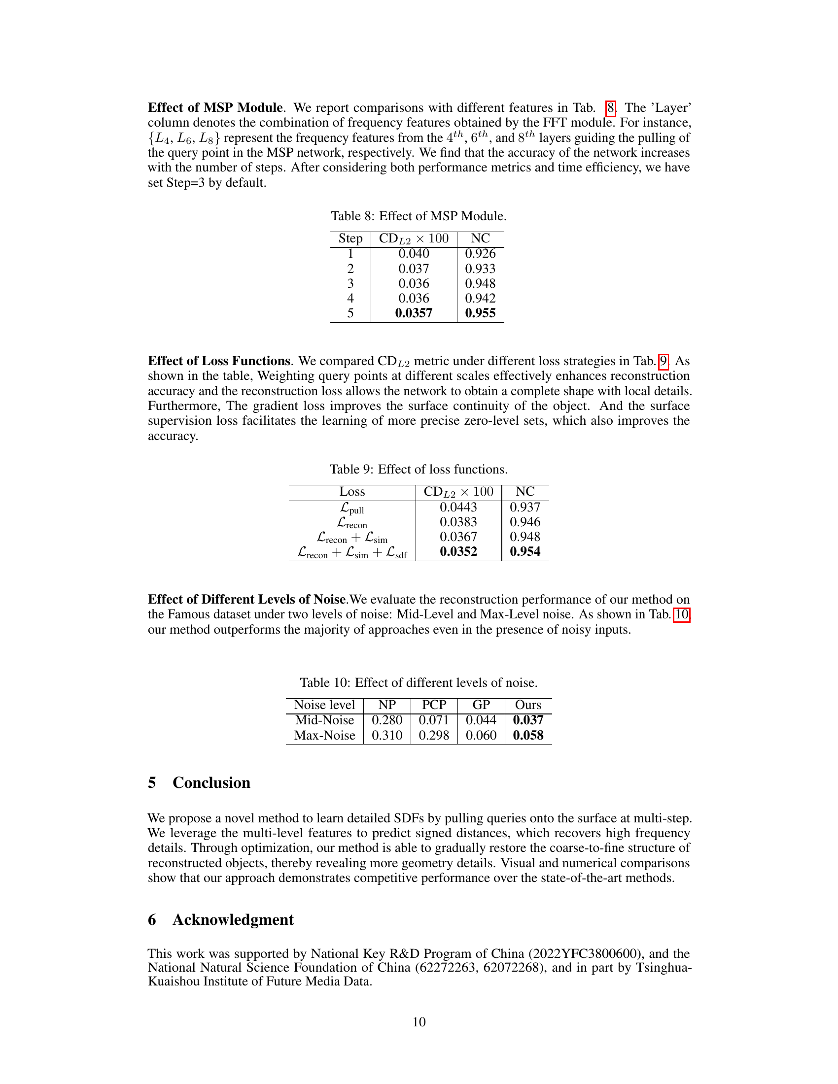
This table shows the effect of varying the number of steps in the Multi-Step Pulling (MSP) module on the reconstruction accuracy. The metrics used are CDL2 (Chamfer Distance L2) and NC (Normal Consistency). As the number of steps increases from 1 to 5, both CDL2 and NC improve, indicating better reconstruction accuracy. However, the gains diminish after 3 steps, suggesting a balance point between accuracy and computational cost.

This table shows the ablation study of different loss functions used in the MultiPull model. The results are presented in terms of CDL2 × 100 and NC (Normal Consistency) metrics. It demonstrates how different combinations of losses (Lpull, Lrecon, Lsim, Lsdf) impact the final reconstruction quality. The best performance is achieved using the combination of all loss functions.

This table shows the reconstruction accuracy (CDL2) of different methods (NP, PCP, GP, and Ours) under two noise levels: Mid-Noise and Max-Noise. It demonstrates the robustness of the proposed MultiPull method to noise compared to other state-of-the-art methods.
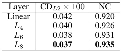
This table presents the ablation study on the effect of using different numbers of frequency layers in the Frequency Feature Transformation (FFT) module of the MultiPull model. It compares the performance using only one layer (L4), combinations of layers (L4,L6), and (L4,L6,L8) against a baseline using only linear layers. The results show that using higher-level frequency layers improves the reconstruction accuracy, measured by both CDL2 and NC.

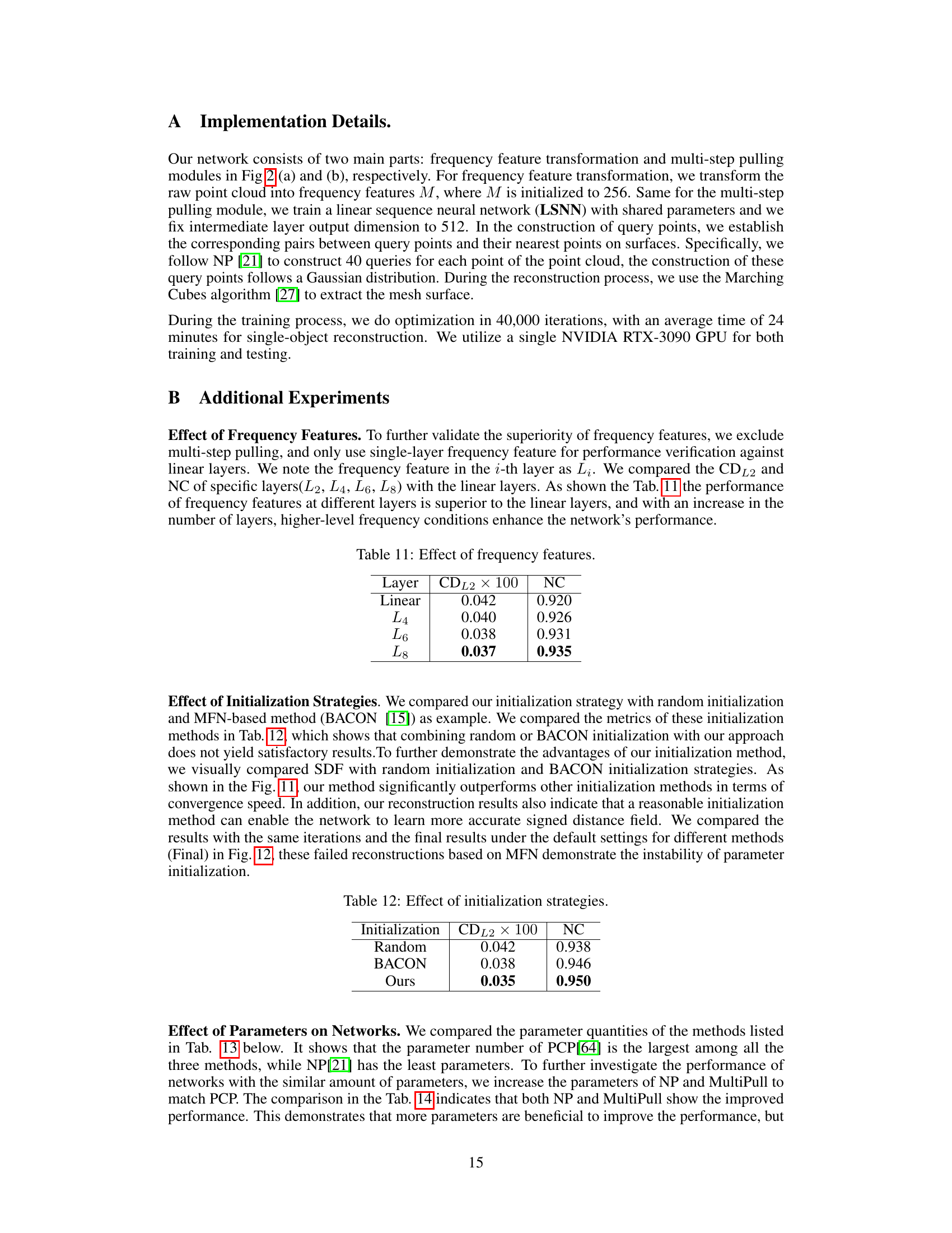
This table presents a comparison of reconstruction accuracy using different initialization strategies for the neural network. The metrics used are Chamfer Distance (CDL2) and Normal Consistency (NC). The results show that the proposed initialization method outperforms random and BACON initialization strategies in terms of both CDL2 and NC.

This table presents a comparison of the proposed MultiPull method against several state-of-the-art techniques for surface reconstruction on the FAMOUS dataset. The metrics used are the Chamfer Distance (CDL2), which measures the average distance between the reconstructed and ground truth surfaces, and Normal Consistency (NC), which assesses the alignment of surface normals. Lower CDL2 and higher NC values indicate better reconstruction quality. The table shows that MultiPull significantly outperforms existing methods on this benchmark.

This table compares the performance of three different methods (NP, PCP, and Ours) on the ShapeNet dataset when they have approximately the same number of parameters. The goal is to evaluate whether the superior performance of the ‘Ours’ method is due to the method itself or simply a result of having more parameters. The table shows CDL2 × 100 and NC metrics. The ‘Ours’ method still outperforms the others even with similar parameter counts, suggesting that the method’s design, rather than a higher parameter count, is the key to improved results.

This table compares the inference time of three different methods: PCP, NP, and Ours. The inference time is measured in minutes. The results show that NP has the fastest inference time, followed by Ours and PCP.

This table shows the comparison results of using different loss functions, including
Lgrad(avg)andLgrad(min), in the MultiPull method, along with the baseline (withoutLgrad). The metrics used for comparison are Chamfer Distance (CDL2) and Normal Consistency (NC). The results demonstrate thatLgrad(min)consistently outperforms other options across the two metrics.

This table compares the reconstruction accuracy (CDL2) of different combinations of feature extraction methods (Linear, PointMLP) and pulling methods (Pull, MSP) at different iteration numbers (10K, 20K, 40K). It demonstrates the impact of combining multi-step pulling (MSP) with different feature extractors on the model’s performance in reconstructing surfaces.

This table presents the results of an ablation study that investigated the impact of using different combinations of frequency layers (L4, L6, L8) on the performance of the MultiPull model. The metrics reported are the Chamfer Distance (CDL2) and Normal Consistency (NC), which are commonly used for evaluating surface reconstruction. The table shows that combining multiple layers leads to better accuracy, as evidenced by lower CDL2 and higher NC values. Specifically, the best performance was achieved using layers L4, L6, and L8 together.
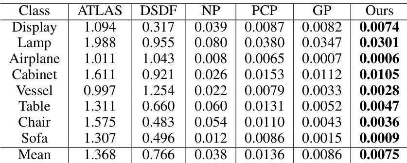
This table presents a quantitative comparison of the proposed MultiPull method against other state-of-the-art techniques for 3D shape reconstruction on the ShapeNet dataset. The evaluation metrics used are Chamfer Distance (CDL2), Normal Consistency (NC), and F-Score, calculated at two different thresholds (0.002 and 0.004). The results demonstrate the superior performance of MultiPull in terms of accuracy and detail preservation compared to the other methods.
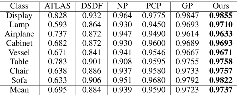
This table presents a quantitative comparison of the MultiPull method against several state-of-the-art techniques for 3D surface reconstruction on the ShapeNet dataset. The evaluation metrics used are Chamfer Distance (CDL2), Normal Consistency (NC), and F-Score at two different thresholds (0.002 and 0.004). Lower values for CDL2 indicate better reconstruction accuracy, while higher values for NC and F-Score represent better normal consistency and surface completeness, respectively.

This table presents the quantitative results of the proposed MultiPull method and compares it with other state-of-the-art methods on the ShapeNet dataset. The metrics used for comparison are Chamfer Distance (CDL2), Normal Consistency (NC), and F-Score (at thresholds of 0.002 and 0.004). These metrics assess the accuracy of surface reconstruction, with lower CDL2 and higher NC and F-Score values indicating better performance.

This table presents the quantitative results of the proposed MultiPull method and several state-of-the-art methods on the ShapeNet dataset. The performance is evaluated using three metrics: Chamfer Distance (CDL2), Normal Consistency (NC), and F-Score. Two different thresholds (0.002 and 0.004) are used for the F-Score metric, providing a more comprehensive evaluation of surface reconstruction accuracy.

This table presents a quantitative comparison of the MultiPull method against several state-of-the-art techniques on the ShapeNet dataset. The comparison is based on three metrics: Chamfer Distance (CDL2), which measures the geometric distance between point clouds; Normal Consistency (NC), which evaluates the alignment of surface normals; and F-Score, which assesses the overall surface reconstruction accuracy at two different thresholds (0.002 and 0.004). Lower values for CDL2 indicate better geometric accuracy, while higher values for NC and F-Score represent better normal consistency and overall shape reconstruction, respectively.
Full paper#
