↗ OpenReview ↗ NeurIPS Homepage ↗ Chat
TL;DR#
Classical optimization theory struggles to explain the success of machine learning optimization and provides limited guidance on step size selection. Existing Bayesian optimization methods, while theoretically sound, are computationally expensive and impractical for high-dimensional problems. This creates a need for new theoretical frameworks that better bridge the gap between theory and practice.
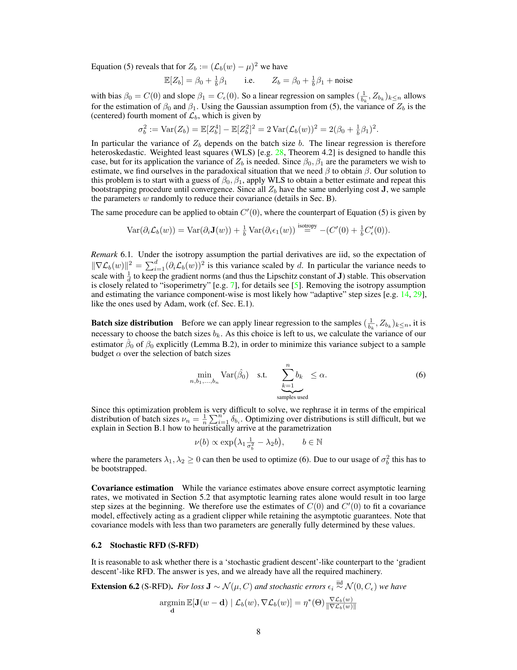
The paper introduces Random Function Descent (RFD), a novel optimization algorithm based on a ‘random function’ framework. RFD rediscovers gradient descent, offering scale invariance and an explicit step size schedule. This framework offers theoretical explanations for established heuristics like gradient clipping and learning rate warmup, overcoming the limitations of previous approaches. Empirical results on the MNIST dataset demonstrate RFD’s effectiveness and efficiency.
Key Takeaways#
Why does it matter?#
This paper is crucial for researchers in optimization and machine learning because it provides a novel theoretical framework for understanding and improving gradient-based optimization methods. It offers scale-invariant algorithms and explains common heuristics, bridging the gap between theoretical optimization and practical applications. This work has significant implications for algorithm development and improving the efficiency and effectiveness of machine learning models.
Visual Insights#

This figure compares three different approximations of a Gaussian random function J(w) around a point w=0. The blue line represents the actual function, the dashed orange line represents the expectation of the function given its value and gradient at w=0, and the solid green line represents a classical Taylor expansion approximation. The shaded area shows the range of possible values of J(w) given the value and gradient at w=0, showcasing that this stochastic Taylor approximation naturally includes a form of trust bound.
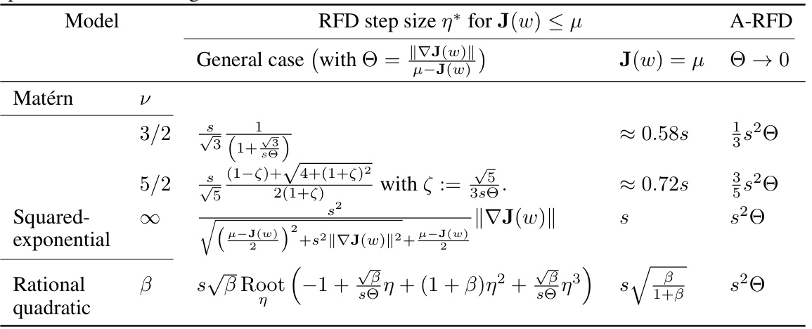
This table presents the formulas for computing the optimal step size (η*) for the Random Function Descent (RFD) algorithm. It shows the general formula and simplified formulas for three different covariance models: Matérn (with ν = 3/2 and ν = 5/2), Squared-exponential, and Rational quadratic. The formulas depend on the gradient norm (||∇J(w)||), the difference between the average cost (μ) and current cost (J(w)), the length scale (s), and the rational quadratic parameter (β). The ‘A-RFD’ column gives the asymptotic step size (as the cost approaches the average, μ).
In-depth insights#
RFD Algorithm#
The Random Function Descent (RFD) algorithm offers a novel approach to optimization by framing the problem within a ‘random function’ framework rather than the traditional ‘convex function’ approach. This shift allows for a more realistic modeling of optimization landscapes often encountered in machine learning, particularly regarding step size selection. RFD’s core innovation is the use of a stochastic Taylor approximation to rediscover gradient descent, providing a theoretical basis for common heuristics like gradient clipping and learning rate warm-up. A key advantage is scale invariance, making RFD robust to various scaling transformations of cost functions and input parameters. The algorithm’s explicit step size schedule, derived from the stochastic Taylor approximation and dependent on the covariance structure of the random functions, contributes to its effectiveness. High dimensional scalability is achieved by leveraging the O(nd) complexity of gradient descent, a significant improvement over Bayesian optimization’s O(n³d³) complexity. However, the algorithm’s reliance on distributional assumptions (typically isotropic Gaussian random functions) is a limitation. Furthermore, its greedy and forgetful nature means classical convergence proofs don’t directly apply, necessitating further theoretical development.
Step Size Schedule#
The paper’s analysis of step size scheduling is a significant contribution, moving beyond classical worst-case optimization theory. Instead of relying on heuristics, the authors introduce a novel framework based on random function descent (RFD). This framework provides a theoretical foundation for common heuristics like gradient clipping and learning rate warmup. The authors derive an explicit step size schedule based on the covariance structure of the random function model. Crucially, the step size schedule displays scale invariance, making it robust to changes in the cost function’s scale and parameterization. The asymptotic analysis reveals a connection to constant learning rates, offering an explanation for the practical success of gradient descent. The RFD framework uncovers an explicit, theoretically justified step size schedule that overcomes the limitations of conventional methods, providing a deeper understanding of optimization processes in high-dimensional spaces.
Covariance Estimation#
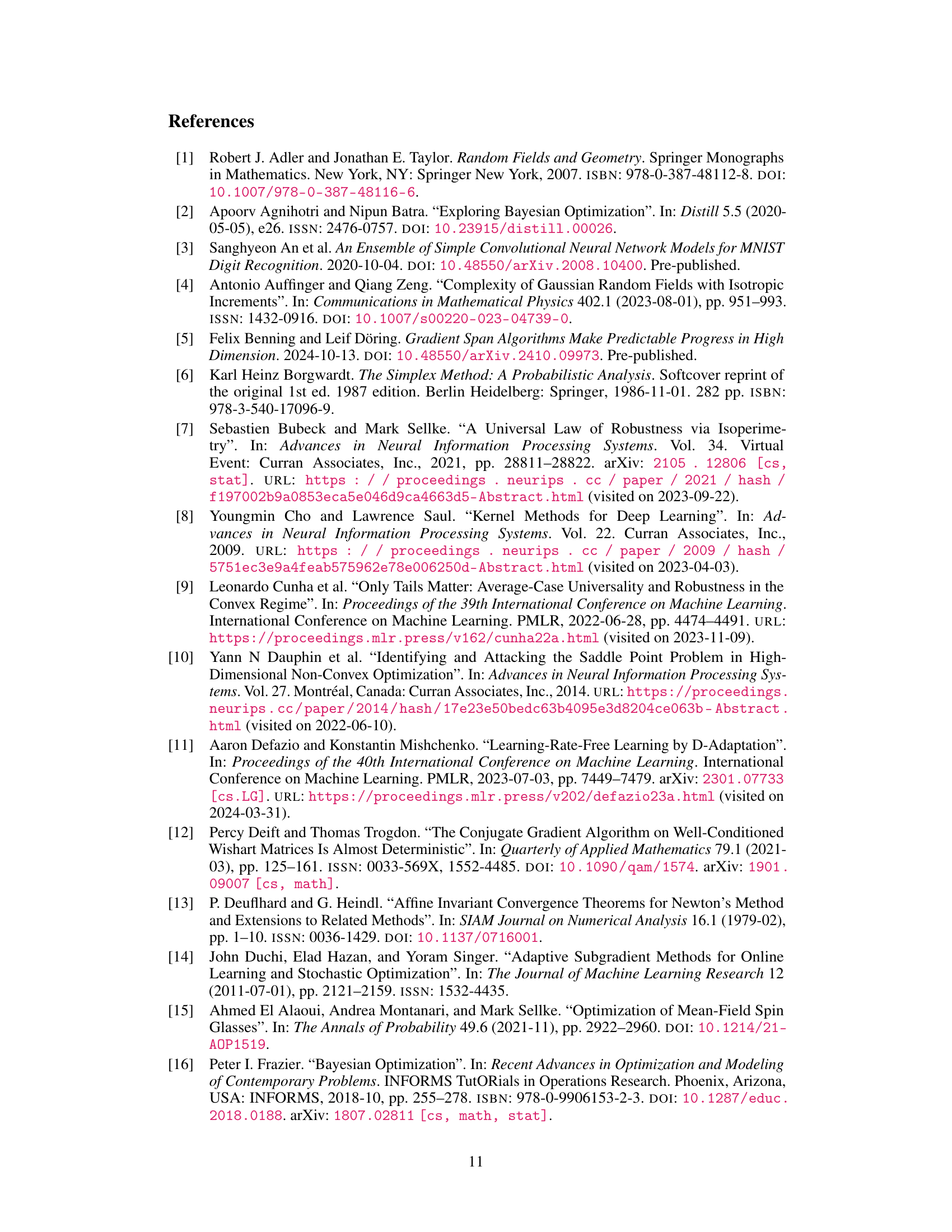
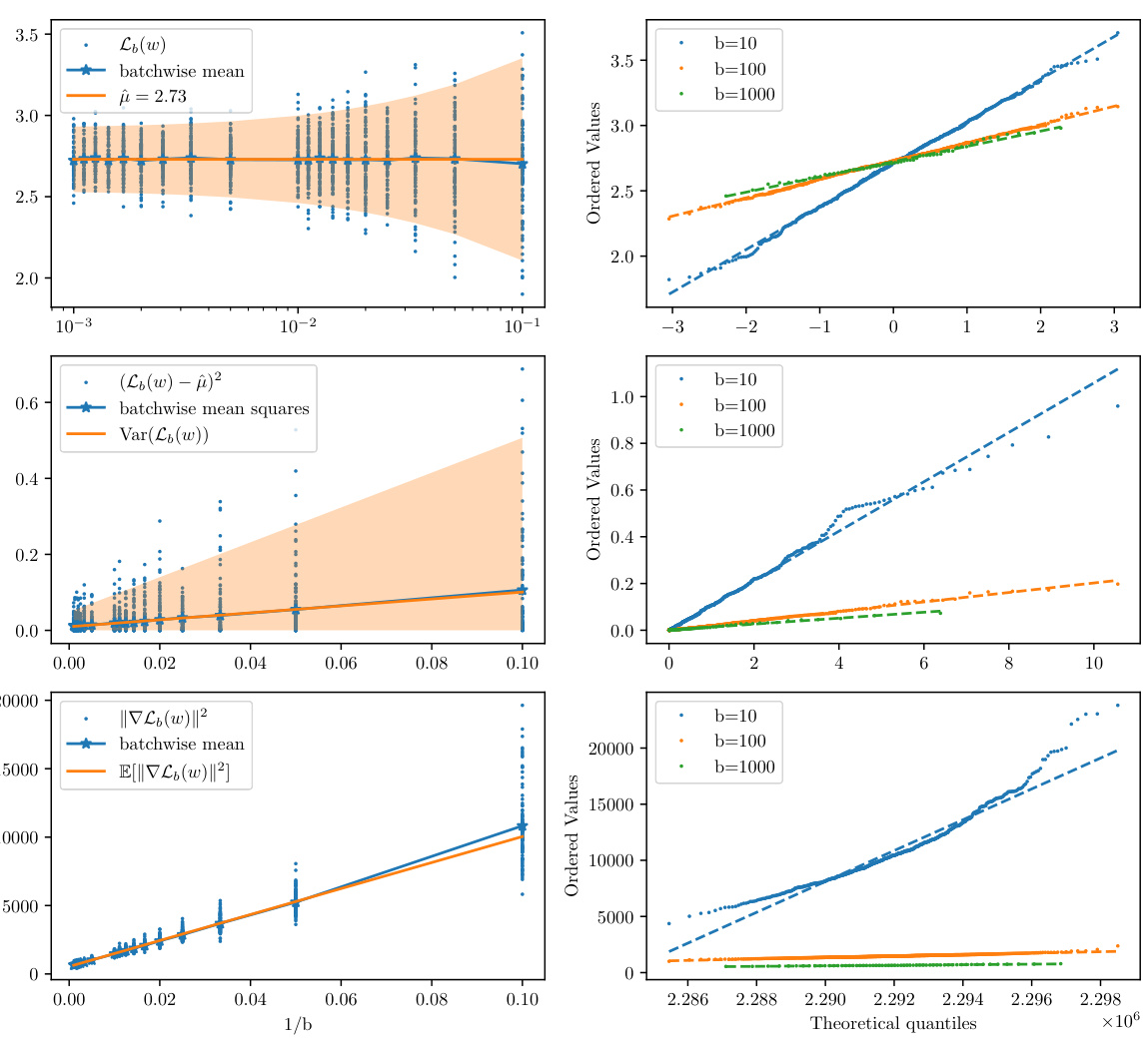
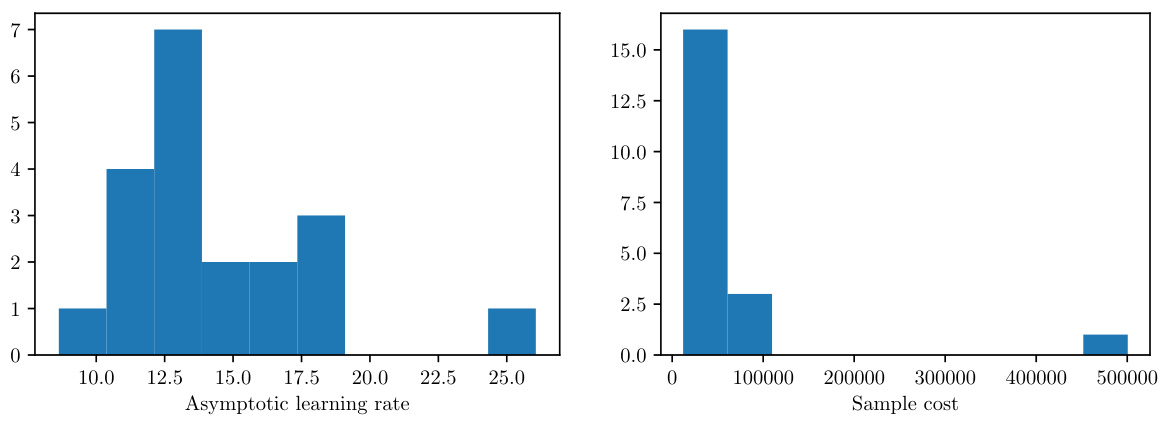
Covariance estimation is crucial for the Random Function Descent (RFD) algorithm, as it directly influences the step size schedule. The authors cleverly tackle the challenge of estimating the covariance matrix without relying on computationally expensive methods. They leverage the isotropy assumption and estimate only C(0) and C’(0), which are sufficient to determine the asymptotic learning rate. A non-parametric variance estimation method is proposed, involving linear regression on samples of the mini-batch losses and their derivatives to provide robust estimates, and making RFD scalable to high-dimensional settings. A crucial aspect is the use of weighted least squares (WLS) to address heteroscedasticity issues inherent in the approach. This robust estimation process, coupled with an iterative bootstrapping procedure, ensures accurate and efficient computation of the required covariance parameters despite the high dimensionality of the data and model complexities. The focus on asymptotic learning rates enables significant computational savings, compared to traditional Bayesian optimization approaches, which typically require extensive computation of full covariance matrices.
Limitations#
The research paper’s limitations section would ideally delve into the assumptions made and their potential impact. Isotropy, a crucial assumption, warrants scrutiny for its applicability across varied datasets and the consequences of deviation. The methodology’s reliance on Gaussian random functions might restrict generalizability, as real-world cost functions rarely perfectly align with this distribution. While the theoretical underpinnings provide insights, computational complexity is a practical consideration. The evaluation’s use of specific covariance models may not reflect the diversity of scenarios. Furthermore, the asymptotic nature of results is a limitation and the implications of this limitation for realistic use-cases must be explored. The dependence on variance estimations potentially impacting practical applicability and performance is another key concern. Finally, discussion on how the approach handles noise and different levels of data smoothness would also strengthen the limitations analysis and improve the overall clarity of the work.
Future Work#
The authors acknowledge the limitations of their current approach and outline several promising avenues for future research. Generalizing beyond the Gaussian and isotropy assumptions is crucial for broader applicability, which they plan to explore using techniques like the best linear unbiased estimator (BLUE). Addressing the inherent risk-affinity of RFD by incorporating mechanisms to manage variance and incorporate confidence intervals is another key area. Improving the efficiency and scalability of RFD, particularly for high-dimensional data, warrants further investigation. They suggest potentially leveraging ideas from adaptive step size methods. Finally, exploring the interaction between RFD and established techniques like momentum and adaptive learning rates could lead to improved optimization algorithms. These directions encompass both theoretical advancements and practical improvements.
More visual insights#
More on figures
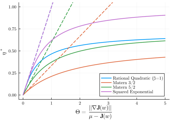
This figure shows the RFD step sizes for four different covariance models as a function of the gradient cost quotient, Θ. It demonstrates how the step size changes during the optimization process, starting with large steps at the beginning and converging to smaller, more constant steps as optimization proceeds. The dashed lines represent the asymptotic RFD (A-RFD), showing the behavior when the optimization is nearly complete. Note that for the rational quadratic covariance model, A-RFD coincides with the A-RFD of the squared exponential covariance model.
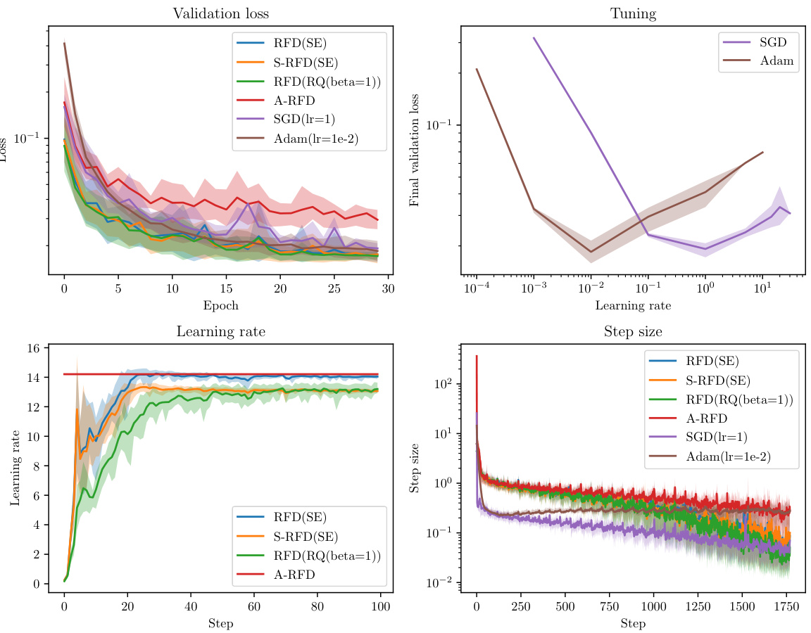
This figure compares the performance of RFD with different covariance functions (squared exponential and rational quadratic) against Adam and SGD optimizers on the MNIST dataset. It shows the validation loss, learning rate, and step size over epochs and steps. The ribbons indicate the variability across 20 repeated experiments, highlighting the robustness and stability of RFD. The results show that RFD, particularly with the squared exponential covariance, exhibits performance comparable to or better than the tuned Adam and SGD optimizers.
This figure shows the training results on the MNIST dataset using different optimization algorithms, namely RFD (with squared exponential and rational quadratic covariance), S-RFD, A-RFD, SGD, and Adam. The results are presented with error bars showing the 10th and 90th percentiles across 20 repeated experiments. The figure illustrates the validation loss and the learning rate/step size for each algorithm over epochs and steps. The key takeaway is that RFD with proper covariance models and step size scheduling outperforms other methods, even showing a form of gradual learning rate warmup.
This figure shows the training results of different optimization algorithms on the MNIST dataset. The algorithms compared are RFD (with squared exponential and rational quadratic covariance), S-RFD (stochastic RFD), Adam, and SGD. The results are visualized using ribbons to show the 10th and 90th percentiles of the results from 20 repeated experiments, giving a sense of the variability. The mean performance is plotted as a line within the ribbon. The figure includes plots of the training loss, validation loss, learning rates, and step sizes over time (epochs and steps). The authors note that the validation loss uses the test data set which gives Adam and SGD a slight advantage since the test set is also used for hyperparameter tuning.

This figure compares the performance of RFD (with squared exponential and rational quadratic covariance) against Adam and SGD optimizers on the MNIST dataset. It shows validation loss, final validation loss, learning rate, and step size across epochs and steps. Ribbons represent the variability (10th-90th percentile) across 20 repeated experiments. The results indicate RFD’s competitive performance, especially considering its automatic step size selection compared to the tuned hyperparameters of Adam and SGD.
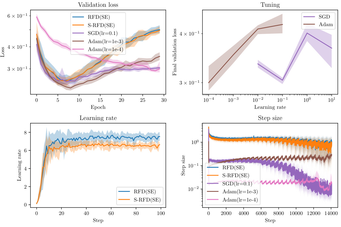
This figure displays the results of training a neural network on the MNIST dataset using different optimization methods: RFD (with squared exponential and rational quadratic covariance), S-RFD, A-RFD, SGD, and Adam. The performance is evaluated using validation loss and learning rate/step size across epochs and steps. The shaded areas (ribbons) represent the variability in the results across multiple runs. The results show that RFD exhibits competitive performance with proper step size management and is superior to A-RFD, highlighting the benefits of the learning rate warmup heuristic.
Full paper#
