Soft ascent-descent as a stable and flexible alternative to flooding

↗ OpenReview ↗ NeurIPS Homepage ↗ Chat

TL;DR

#

Key Takeaways

#

Why does it matter?

#

This paper is crucial for researchers working on generalization in machine learning because it introduces a novel method, SoftAD, that effectively addresses the challenges of high test error and model complexity. The findings offer new avenues for improving model performance and could significantly impact various deep learning applications. Its focus on achieving a balance between accuracy, loss, and model norms opens exciting opportunities for future research. Furthermore, it provides valuable insights into understanding and improving the generalization capabilities of machine learning models.

Visual Insights

#

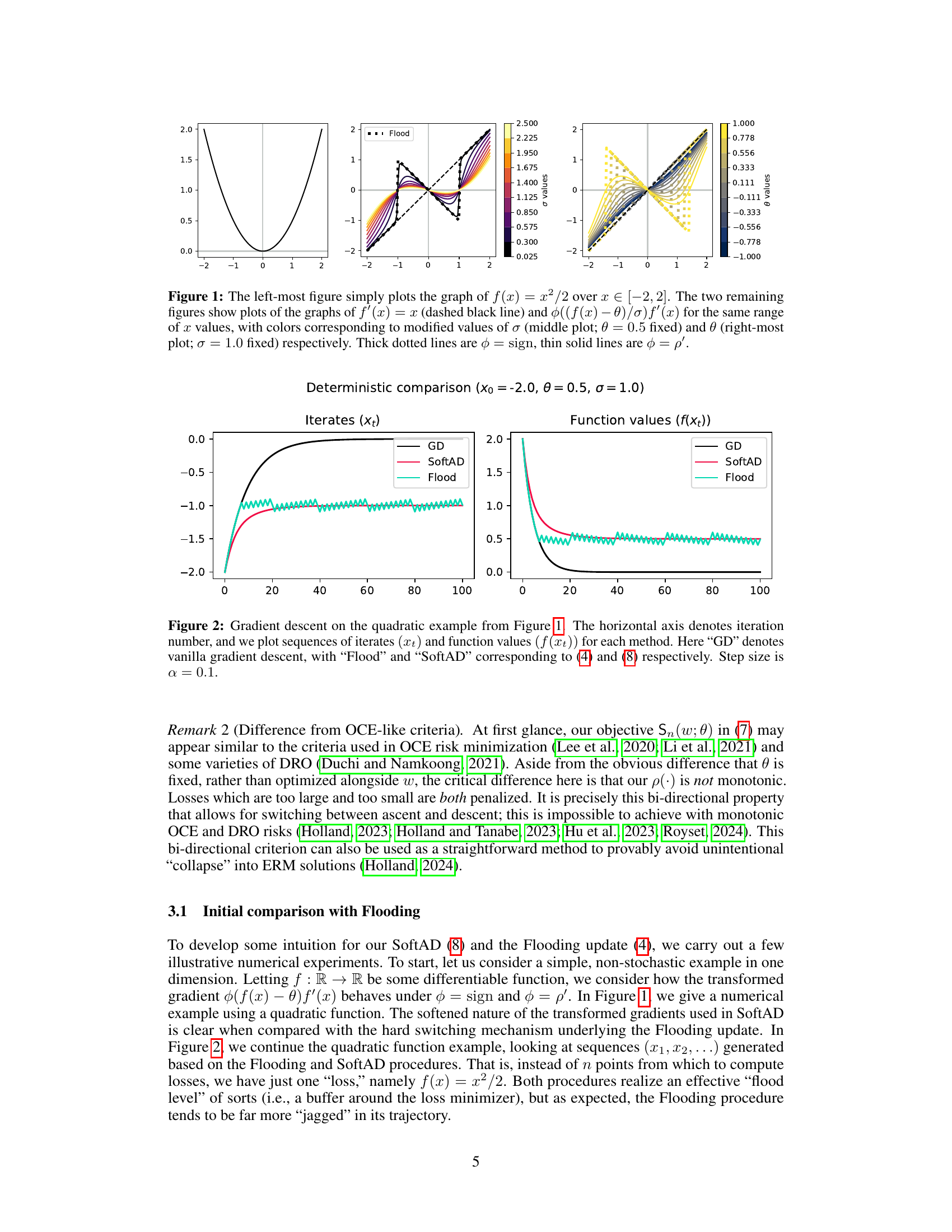
This figure compares the gradients of the quadratic function f(x) = x²/2 with its modified version, where the modification involves scaling and shifting by parameters θ and σ. The leftmost plot shows the quadratic function. The middle plot compares the gradients for different values of σ, while keeping θ fixed. The rightmost plot compares the gradients for different values of θ, while keeping σ fixed. In each case, the effect of the SoftAD’s smooth truncation function φ(x) = x/√x²+1 is demonstrated, showing how it contrasts with the sharp thresholding used in the original Flooding algorithm.

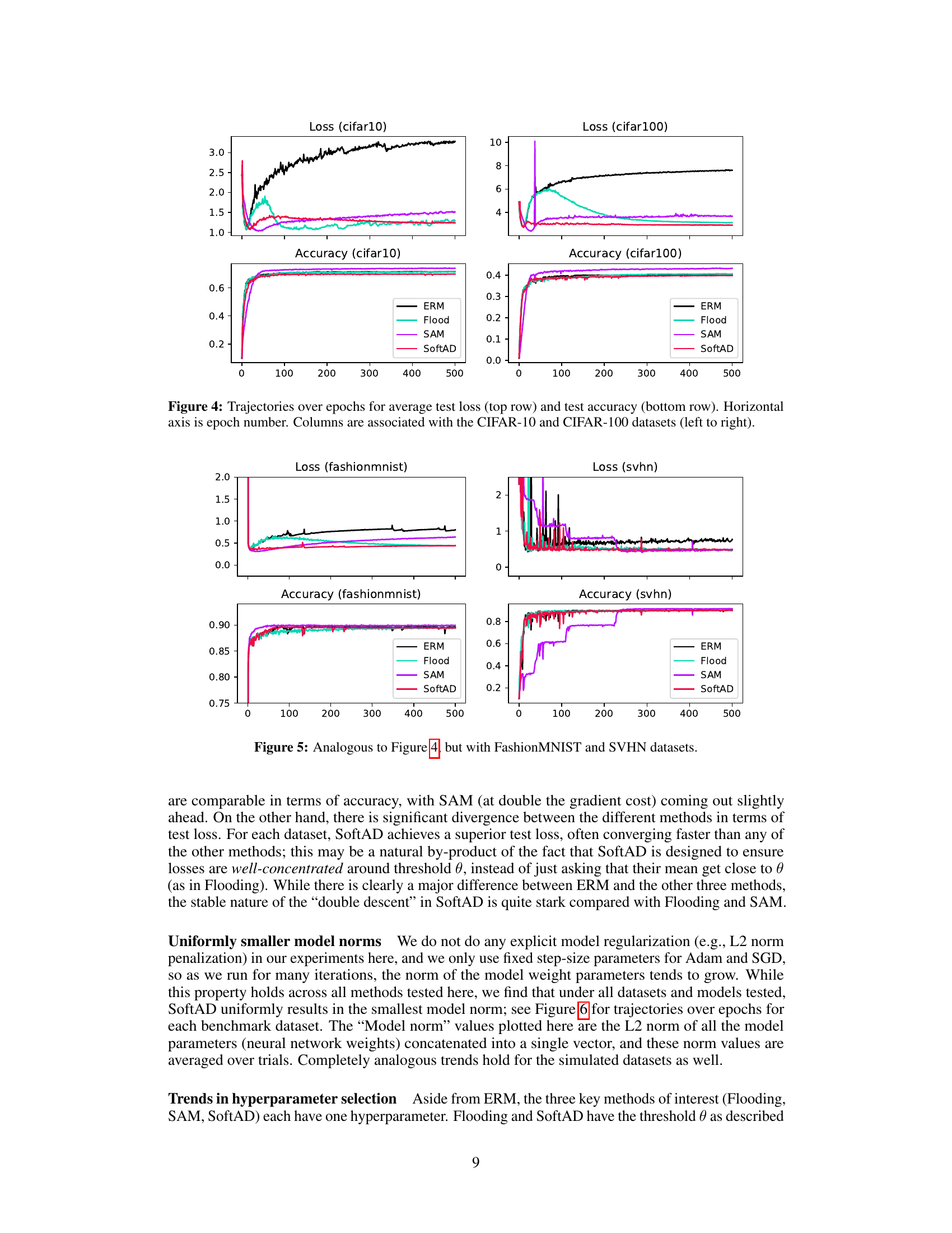
This table shows the difference between the test and training cross-entropy loss for four different methods (ERM, Flood, SAM, SoftAD) across several datasets (Gaussian, Sinusoid, Spiral, CIFAR-10, CIFAR-100, Fashion, SVHN). A smaller value indicates better generalization. The results are averaged over multiple trials, and the cross-entropy loss is calculated after the final training epoch.

In-depth insights

#

SoftAD vs. Flooding

#

The core difference between SoftAD and Flooding lies in their approach to loss manipulation during training. Flooding uses a hard threshold, switching between gradient ascent and descent based on whether the average training loss is above or below a predefined value. This abrupt switching can lead to instability and sensitivity to the threshold’s precise value. In contrast, SoftAD employs a soft thresholding mechanism, using a smooth function to gradually modulate the update direction based on the individual loss of each data point. This approach offers greater stability and robustness, reducing the impact of outliers and providing smoother convergence. SoftAD’s pointwise thresholding allows for a more nuanced response to the loss landscape, combining ascent and descent updates in a more balanced way. This subtle difference has significant consequences; SoftAD demonstrates smaller generalization error and model norms compared to Flooding, while maintaining competitive accuracy. Empirically, SoftAD proves to be a more flexible and stable alternative to Flooding, highlighting the advantages of a softened approach to loss manipulation.

Sharpness & Generalization

#

The relationship between sharpness and generalization in machine learning is complex and not fully understood. Sharpness, often measured by the curvature of the loss function around a minimum, intuitively suggests that flatter minima lead to better generalization. However, empirical evidence shows that this isn’t always the case, and sharp minima can sometimes generalize well. This suggests that other factors influence generalization, possibly including the model’s capacity, data distribution, and the optimization algorithm used. The concept of loss landscape geometry plays a crucial role, highlighting how the distribution of minima and saddle points within the landscape can affect the optimization process and, ultimately, generalization. Regularization techniques, such as weight decay, help to induce flatter minima, often improving generalization. However, there’s a trade-off between sharpness and other performance metrics, such as training accuracy and computational cost. Therefore, the best approach for improving generalization remains an area of active research, requiring a nuanced understanding of the interplay between various factors contributing to model performance.

Empirical Results

#

An Empirical Results section in a research paper would ideally present a comprehensive evaluation of the proposed method against established baselines. Clear visualizations (graphs, tables) are crucial for showcasing the performance metrics (accuracy, loss, etc.) across various datasets. Statistical significance testing should be used to determine if observed differences are meaningful. The discussion of results should go beyond simply reporting numbers; it should provide a thoughtful analysis, highlighting both strengths and weaknesses of the proposed method in relation to the baselines. Key factors affecting performance, such as hyperparameters, model architecture, dataset characteristics, should be explored and discussed. The analysis should address the generalizability of findings, exploring whether observed trends hold under varied conditions. Finally, any unexpected or surprising results deserve focused attention and potential explanations.

Convergence Analysis

#

A rigorous convergence analysis is crucial for evaluating the reliability and efficiency of any machine learning algorithm. For the SoftAD algorithm, such an analysis would ideally establish formal guarantees on the algorithm’s convergence to a stationary point of the objective function. This would likely involve demonstrating that the iterates generated by SoftAD satisfy specific conditions, such as boundedness and sufficient decrease. The smoothness properties of the objective function and the choice of step size would play a key role in determining the convergence rate. A comparison with the convergence properties of existing algorithms, such as flooding and SAM, would highlight the advantages and disadvantages of SoftAD. Establishing tighter bounds on the convergence rate could significantly enhance the theoretical understanding of SoftAD’s performance. Furthermore, investigating whether the algorithm converges to a global or local minimum would provide valuable insights. Finally, a detailed analysis of the impact of hyperparameters on the convergence behavior is vital for practical applications.

Future Work

#

Future research directions stemming from this work could explore several avenues. Investigating alternative smooth truncation functions beyond the chosen ρ(x) could reveal improved performance or theoretical guarantees. Developing principled methods for setting the threshold parameter θ is crucial, perhaps leveraging Bayesian approaches or techniques for estimating the Bayes error to connect this parameter to a desired level of accuracy. Furthermore, a more in-depth theoretical analysis could explore the relationship between the SoftAD’s pointwise mechanism and implicit regularization. Finally, examining the method’s effectiveness across a broader range of model architectures and datasets, including those involving high-dimensional data and more complex tasks, is vital to ascertain its general applicability and potential limitations.

More visual insights

#

More on figures

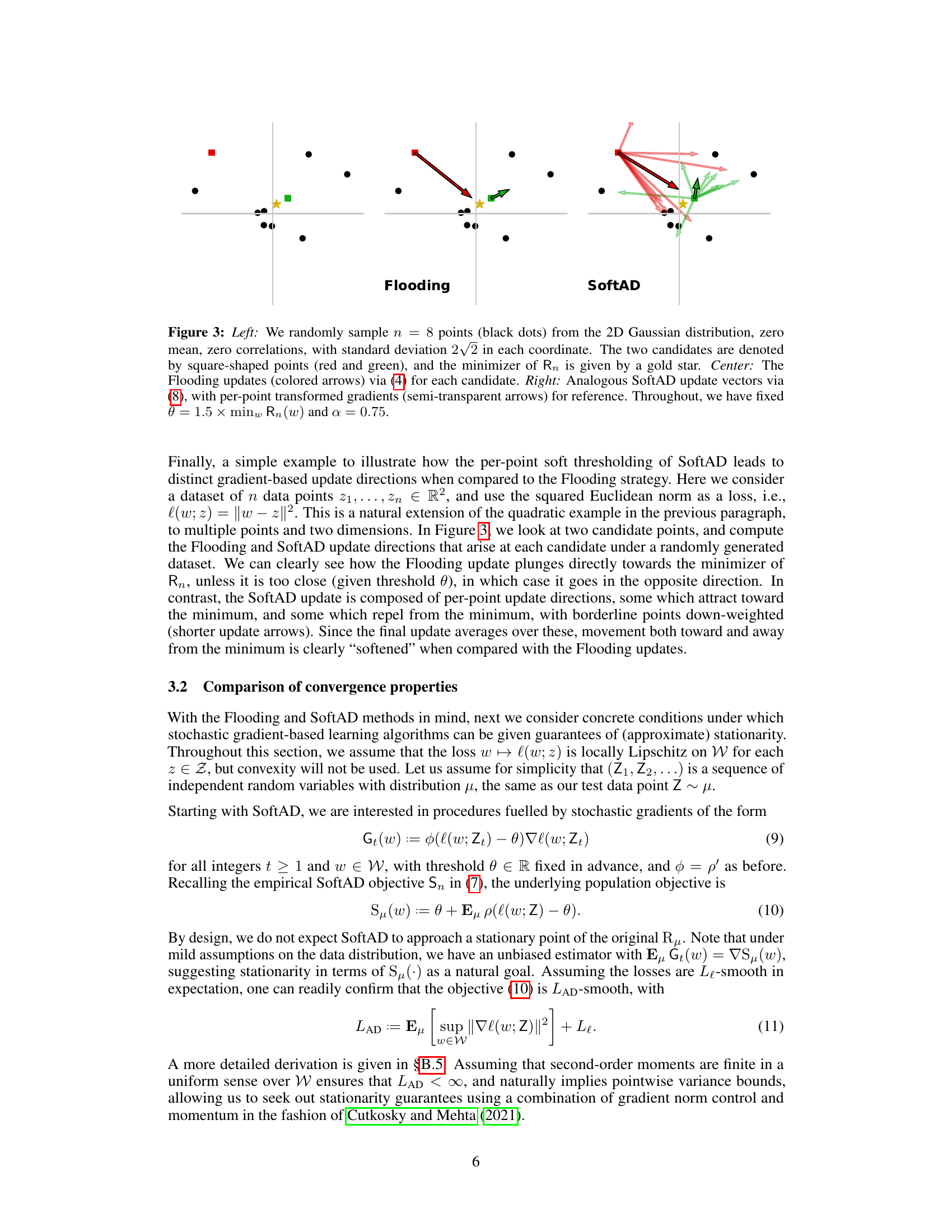
This figure compares the performance of vanilla gradient descent (GD), Flooding, and SoftAD on a simple quadratic function. The x-axis represents the iteration number, and the y-axes show the iterates (x_t) and function values (f(x_t)) respectively. The plot demonstrates that SoftAD converges more smoothly than Flooding, which oscillates near the minimum, while GD approaches the minimum directly.

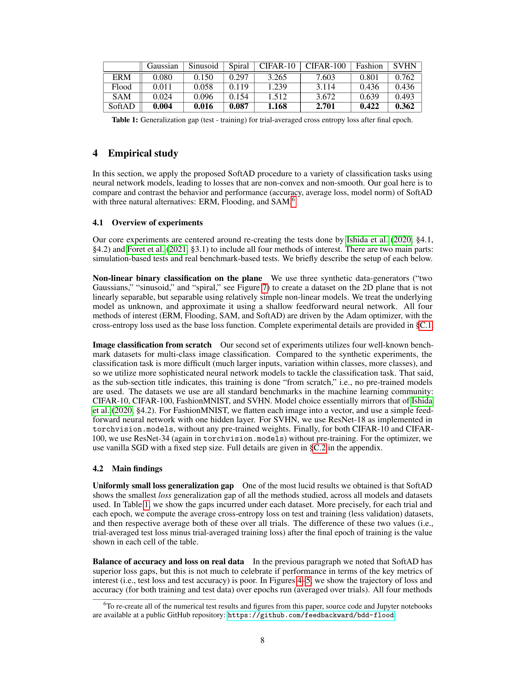
This figure compares the update directions of Flooding and SoftAD. In the left panel, eight data points are sampled from a 2D Gaussian distribution, with two candidate points (red and green squares) and the empirical risk minimizer (gold star). The center panel shows the Flooding update vectors for each candidate, illustrating a direct movement towards or away from the minimizer. The right panel demonstrates SoftAD updates, which involve per-point update directions (semi-transparent arrows) that are weighted and aggregated, resulting in a smoother and more nuanced update compared to Flooding.

This figure shows the training curves for test loss and accuracy using four different methods: ERM, Flooding, SAM, and SoftAD. The curves are plotted against the number of training epochs. The figure is split into two columns, one for the CIFAR-10 dataset and the other for CIFAR-100 dataset. Each column has two subplots, the upper one for loss and the lower one for accuracy. The plots visualize the performance of each method over the course of training, highlighting the differences in their convergence behavior and final performance.

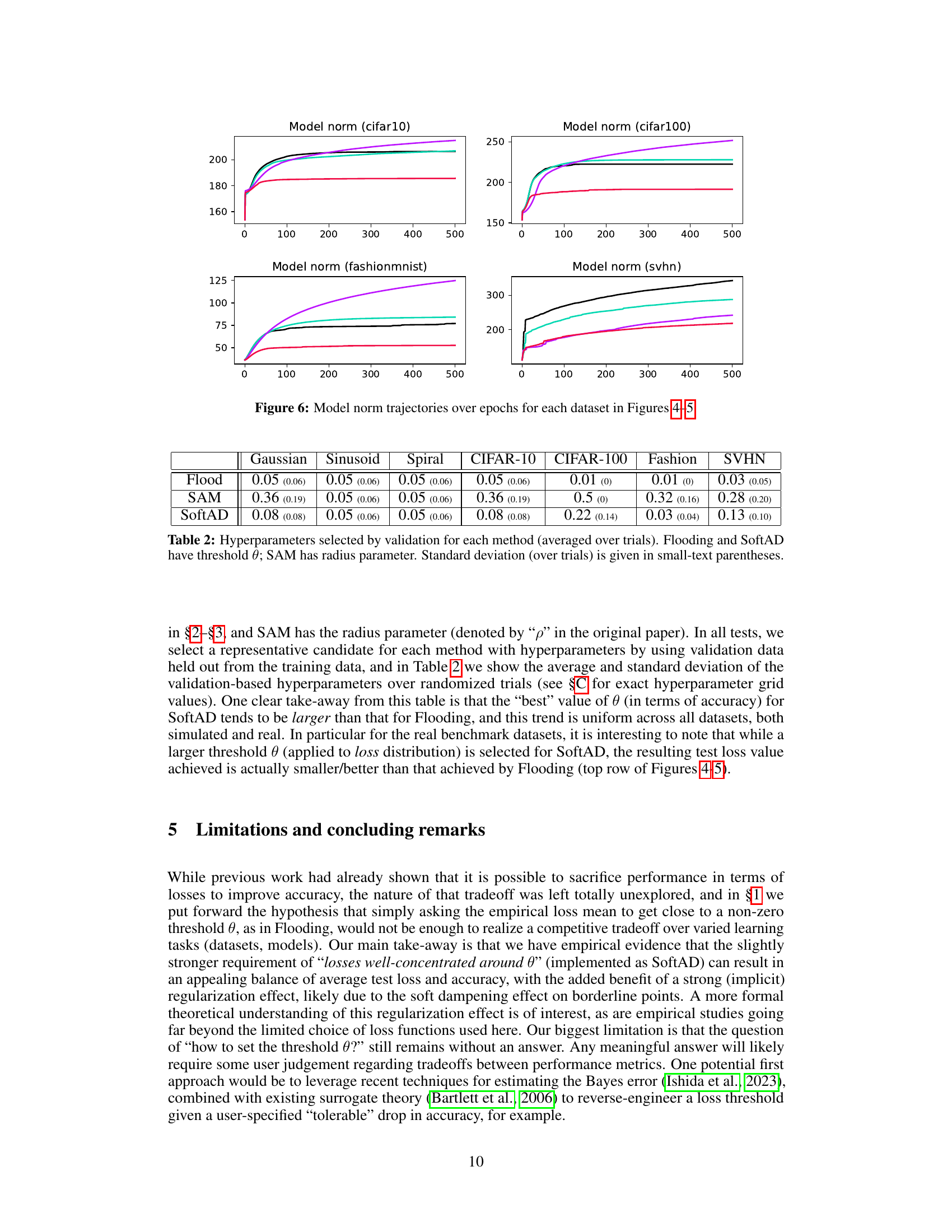
This figure shows the trajectories of model norms over epochs for each dataset used in Figures 8 and 9. The model norm is calculated as the L2 norm of all model parameters concatenated into a single vector. The plots show the average model norm across multiple trials for each method (ERM, iFlood, SoftAD). The x-axis represents the epoch number, and the y-axis represents the L2 norm of model parameters.

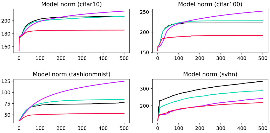
This figure shows the trajectory of model norm (L2 norm of all model parameters) over training epochs for four different datasets (CIFAR-10, CIFAR-100, FashionMNIST, and SVHN) using three methods: ERM, iFlood, and SoftAD. Each line represents one of these methods for a particular dataset. The figure helps to visualize the model norm growth and compare the methods’ effect on model complexity over time. In general, the results show that SoftAD helps to maintain smaller model norms compared to other methods.

This figure shows three synthetic datasets used for binary classification experiments in the paper. Each plot represents a 2D dataset with two classes, shown as circles and crosses. The ’two Gaussians’ dataset shows two overlapping Gaussian distributions. The ‘sinusoid’ dataset shows data points separated by a sinusoidal curve. The ‘spiral’ dataset displays data points forming two intertwined spirals.

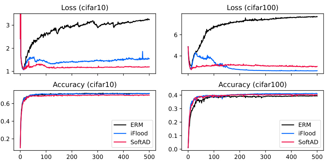
This figure shows the training curves for test loss and accuracy of ERM, iFlood, and SoftAD methods on CIFAR-10 and CIFAR-100 datasets. The top row displays the test loss for each method over training epochs, while the bottom row shows the corresponding test accuracy. It visually demonstrates the performance of each method throughout the training process on these two benchmark image classification datasets.

This figure displays the training trajectories for average test loss and test accuracy over epochs for FashionMNIST and SVHN datasets. It compares four different methods: ERM, iFlood, and SoftAD. The plots show how the training loss and accuracy evolve over time for each method on these datasets, allowing for a visual comparison of their performance characteristics.

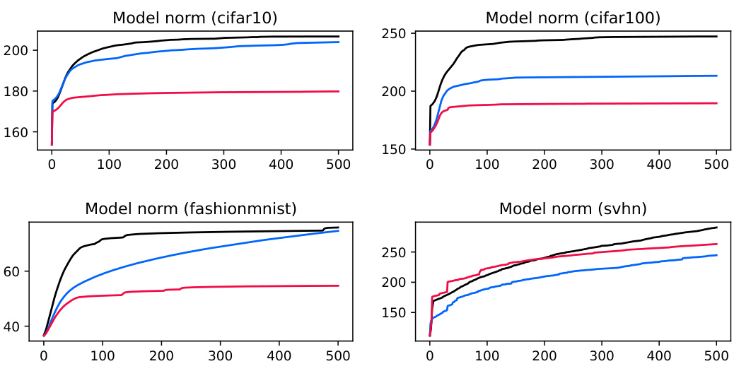
This figure shows the L2 norm of all model parameters (neural network weights) concatenated into a single vector for each dataset (CIFAR-10, CIFAR-100, FashionMNIST, SVHN) over epochs. The norms are averaged over multiple trials for each method (ERM, Flooding, SAM, SoftAD). The figure illustrates that SoftAD consistently maintains smaller model norms compared to the other methods, even without explicit regularization.

This figure compares the performance of ERM, Flooding, and SoftAD on two datasets using a linear model. The left panel shows the average cross-entropy loss over epochs, while the right panel displays the test accuracy. The results indicate that SoftAD can achieve competitive accuracy even at significantly higher loss values than ERM.

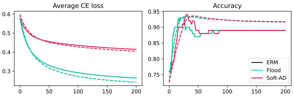
This figure compares the performance of ERM, Flooding, and SoftAD on two datasets using a simple linear model. It shows the average cross-entropy loss and accuracy over 200 epochs. The results illustrate how SoftAD achieves competitive accuracy while maintaining lower average loss compared to ERM and Flooding.

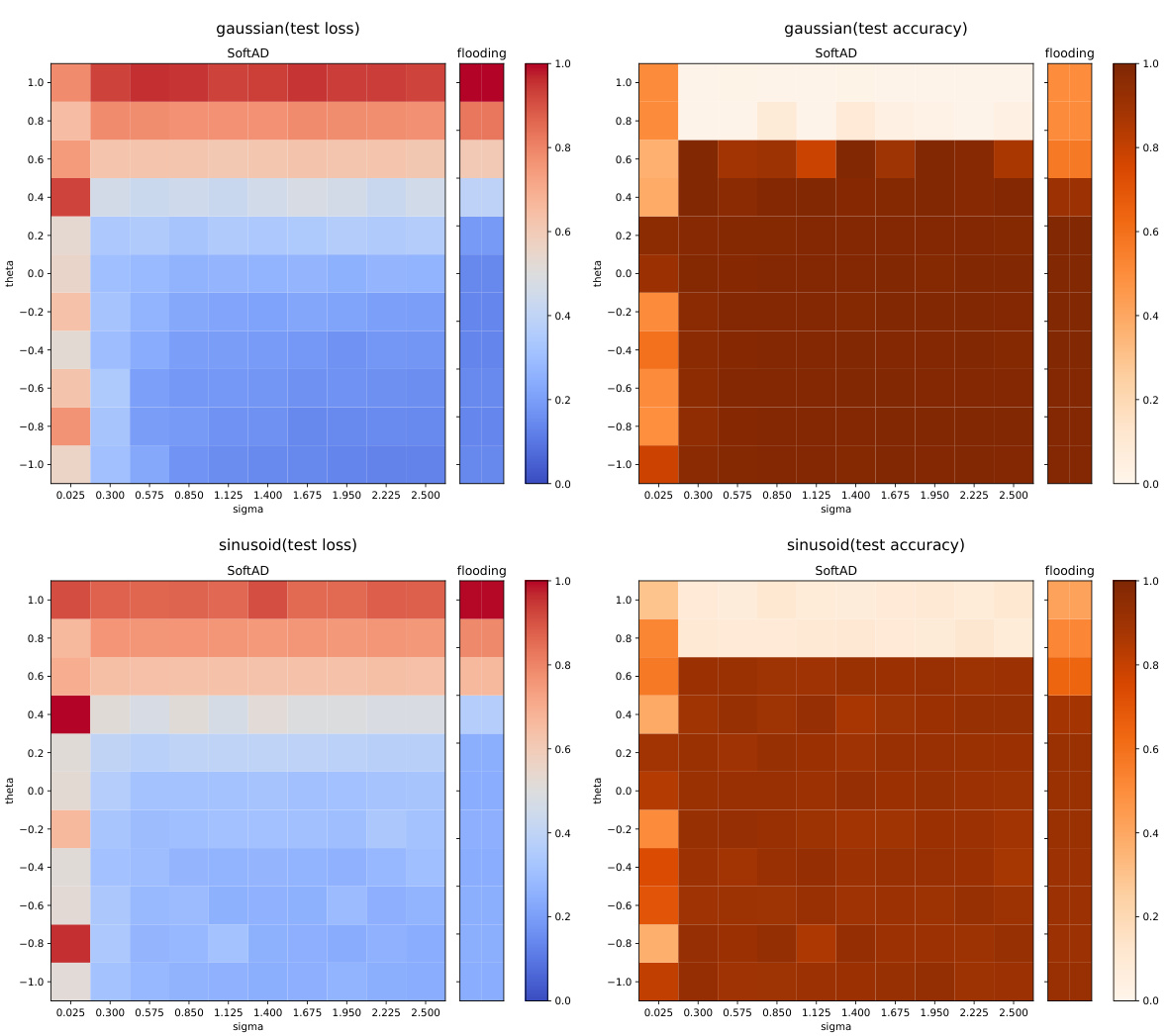
This figure shows heatmaps of test loss and accuracy for both Flooding and SoftAD methods. The heatmaps visualize how the test loss and accuracy change depending on different values of two hyperparameters: the threshold (θ) and the scaling parameter (σ). Each cell in the heatmap represents a combination of θ and σ values, and its color intensity indicates the corresponding test loss or accuracy. This visualization helps to understand the impact of the hyperparameters on the performance of the two methods. The heatmaps are generated separately for two synthetic datasets: ‘gaussian’ and ‘sinusoid’.

More on tables

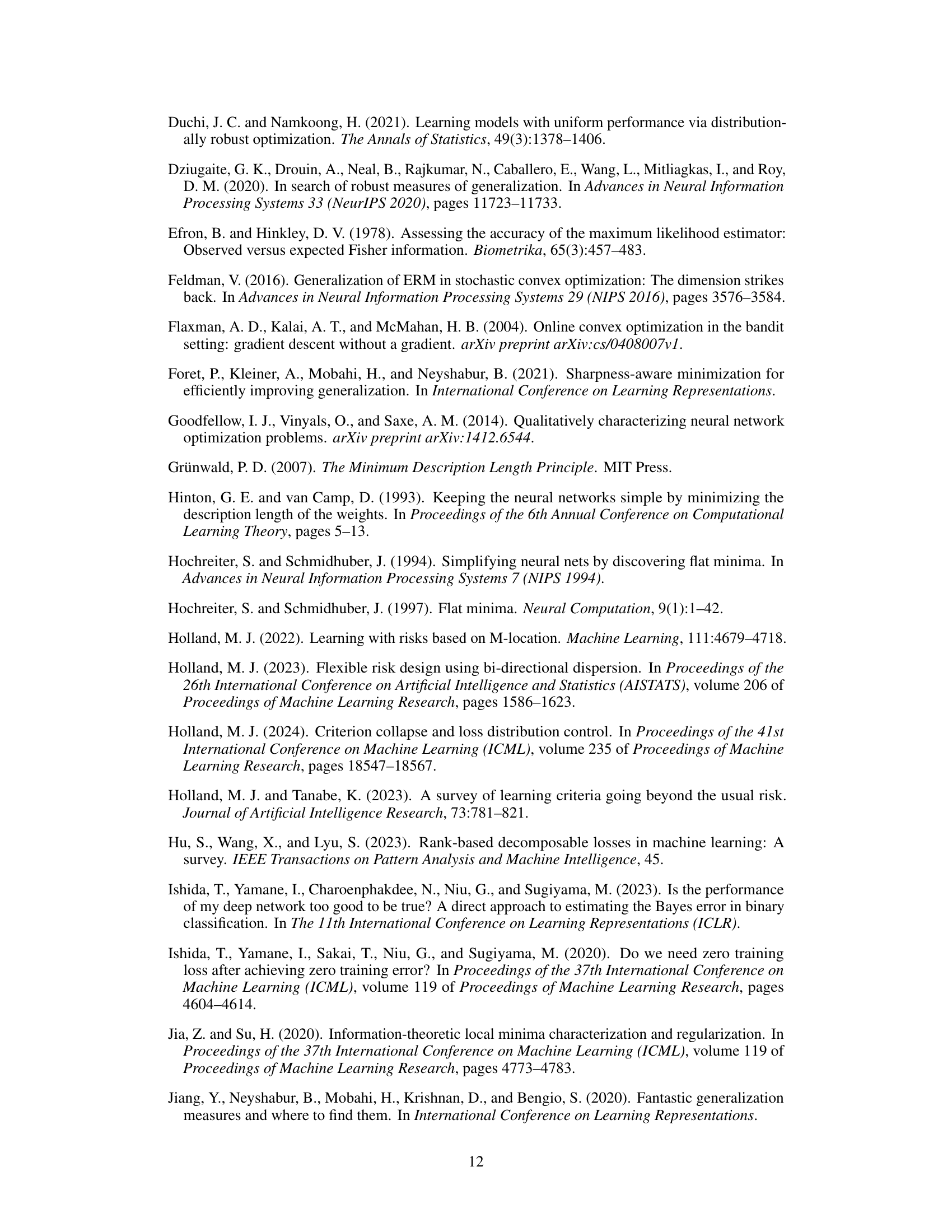
This table presents the hyperparameter settings used for the Flooding, SAM, and SoftAD methods across different datasets. The hyperparameters were selected using validation data to optimize performance. For Flooding and SoftAD, the threshold θ is reported, while for SAM, the radius parameter is shown. Standard deviations across trials are included in parentheses to indicate variability.

This table presents the generalization gap, calculated as the difference between test and training average cross-entropy loss, for three different algorithms: ERM, iFlood, and SoftAD. The results are shown for four different datasets: CIFAR-10, CIFAR-100, Fashion, and SVHN. A lower generalization gap indicates better generalization performance of the model.

This table shows the hyperparameter values selected through validation for the Flooding, SoftAD, and SAM methods. The hyperparameter for Flooding and SoftAD is the threshold θ, while for SAM it is the radius parameter. The values are averages across multiple trials, with standard deviations shown in parentheses.

Full paper

#