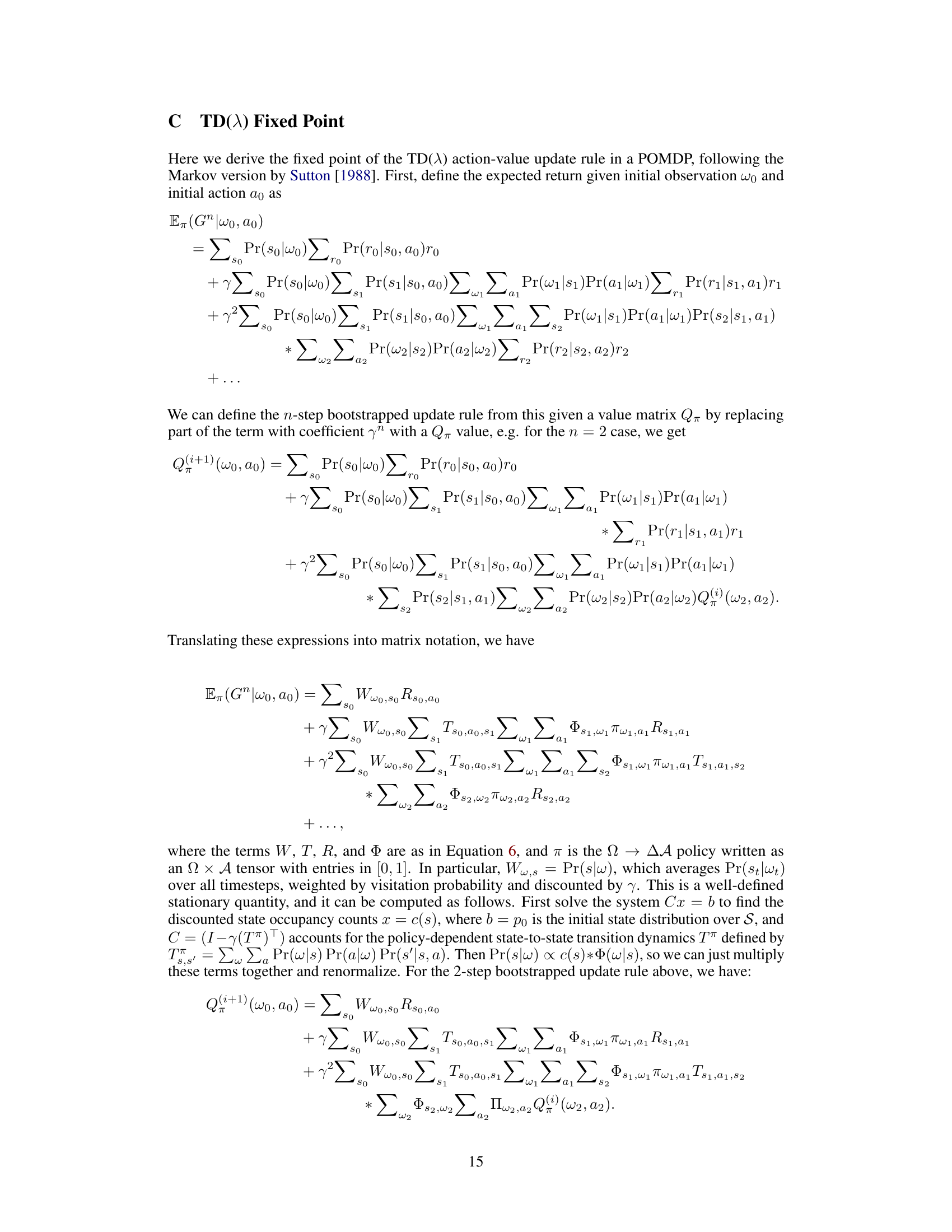
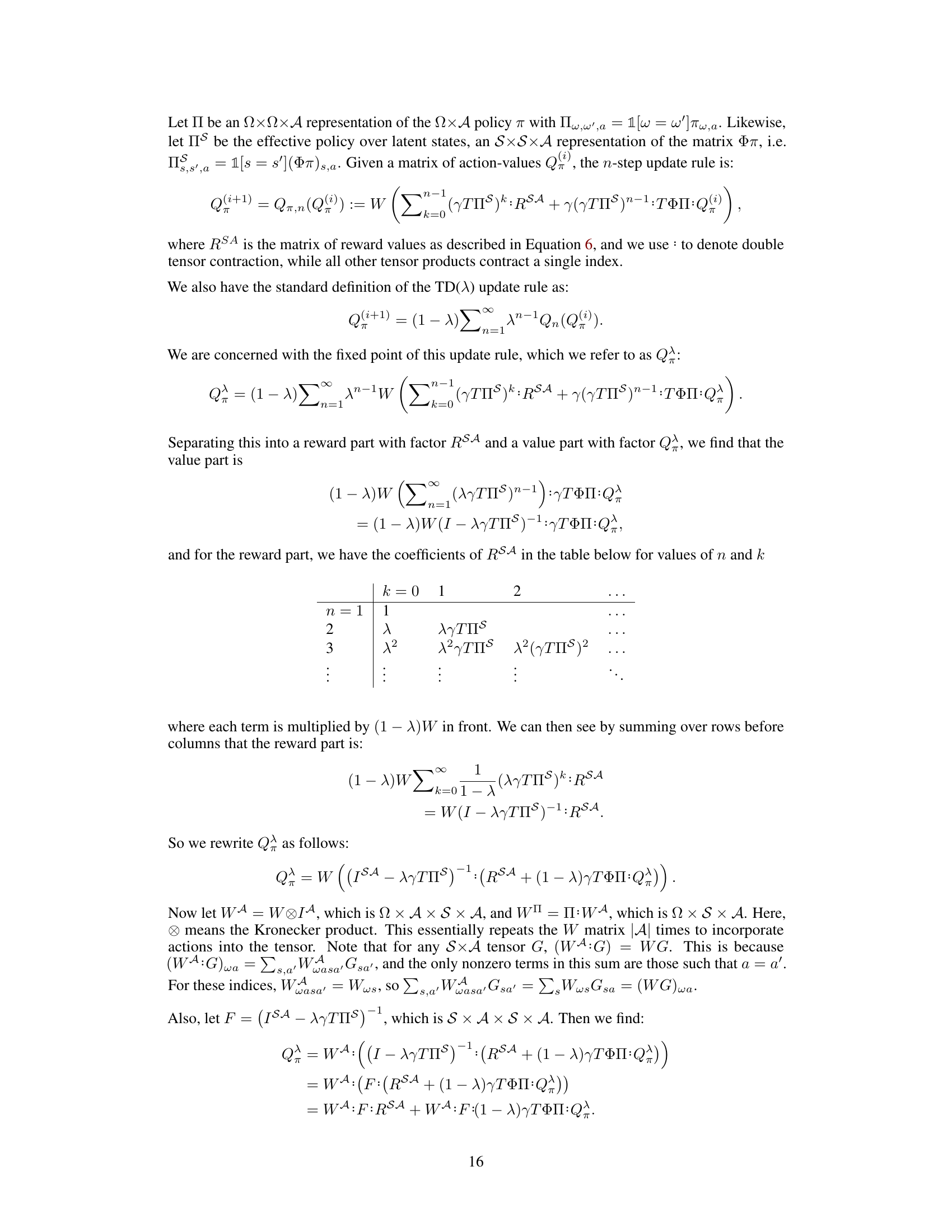
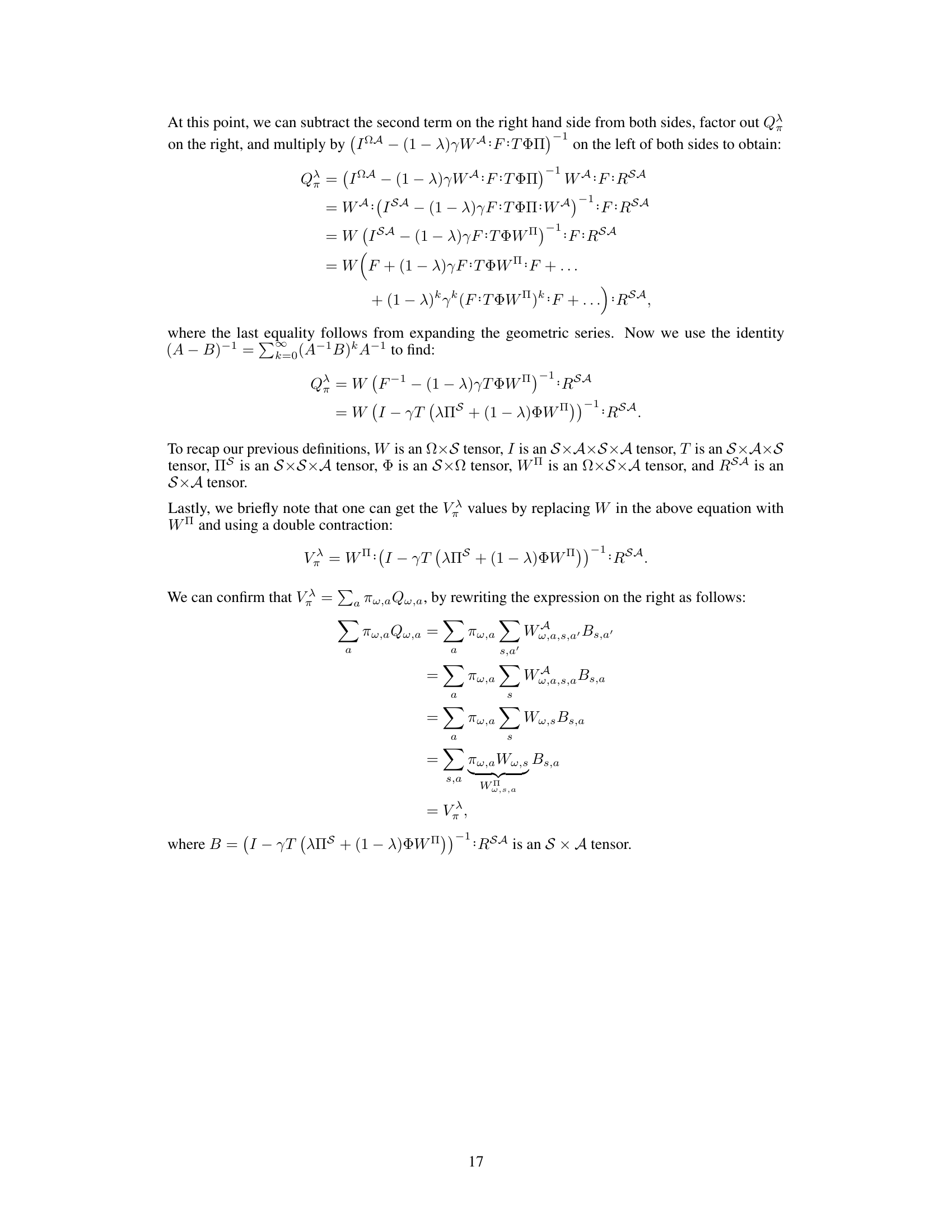
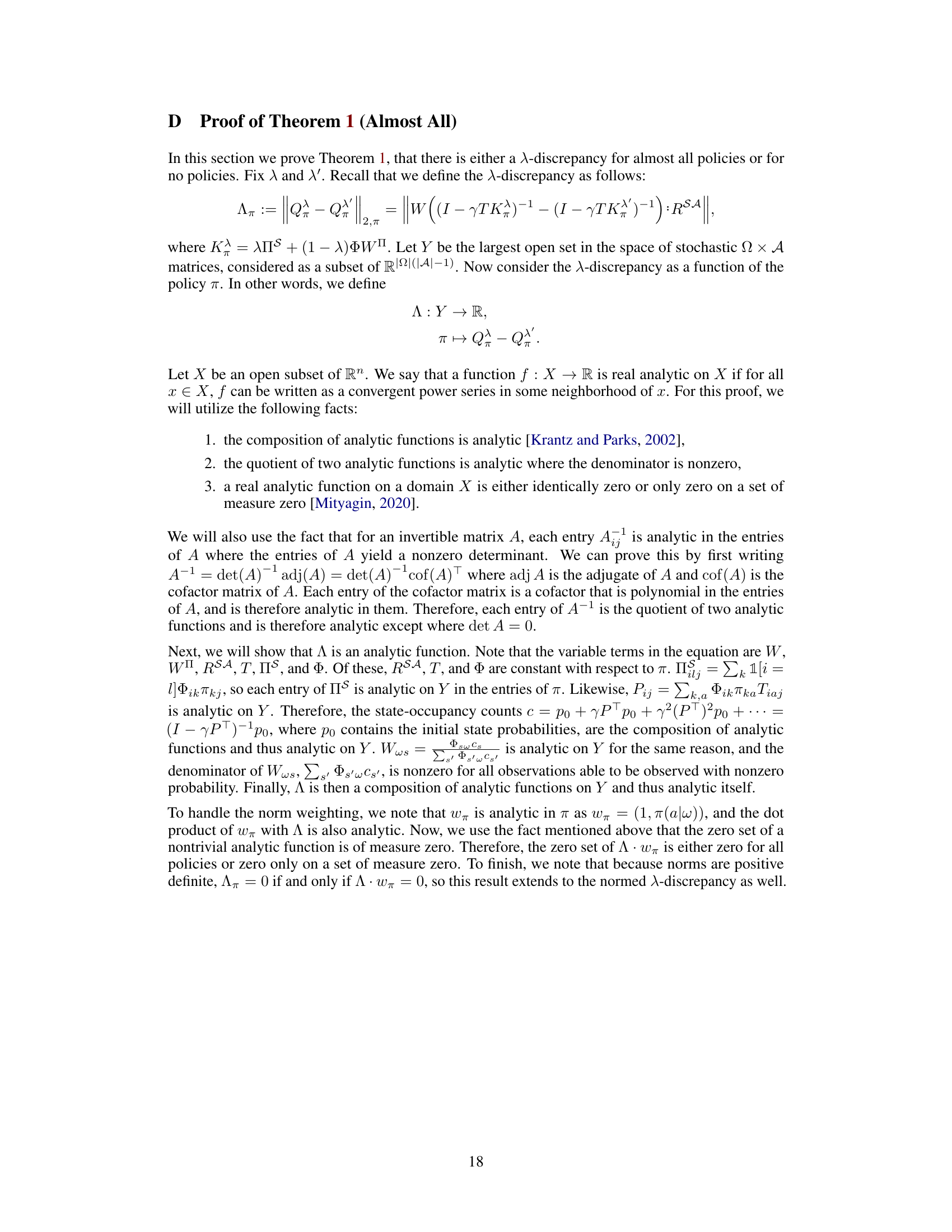
↗ OpenReview ↗ NeurIPS Homepage ↗ Chat
TL;DR#
Many reinforcement learning algorithms assume full observability of the environment. However, real-world scenarios often involve partial observability, where agents only have access to incomplete information about the environment’s state. This limitation significantly hinders the ability of reinforcement learning agents to learn effective policies and achieve optimal performance. Existing methods for handling partial observability often require the explicit knowledge of the underlying state space or involve computationally expensive approaches. This paper addresses the problem by presenting a novel approach.
This research proposes the λ-discrepancy, a metric to quantify the degree of partial observability in an environment. The key idea is comparing value function estimates computed using two different temporal difference (TD) learning methods: TD(λ=0) and TD(λ=1). TD(0) implicitly assumes a Markovian environment, while TD(1) does not. A significant difference between the two estimates suggests non-Markovianity and partial observability. The paper demonstrates how minimizing this discrepancy can improve the performance of reinforcement learning agents, enabling them to handle partially observable environments more effectively. Furthermore, the research showcases that this approach is scalable to complex environments where traditional methods fail. This work provides both a valuable theoretical contribution and a practical algorithm for researchers to leverage in their work.
Key Takeaways#
Why does it matter?#
This paper is crucial for reinforcement learning researchers as it introduces a novel metric for detecting and mitigating partial observability, a significant challenge in real-world applications. The proposed “““λ-discrepancy””” method offers a model-free approach, improving scalability and performance, especially in complex environments. Its applicability to various deep reinforcement learning algorithms makes it a valuable contribution for the field.
Visual Insights#

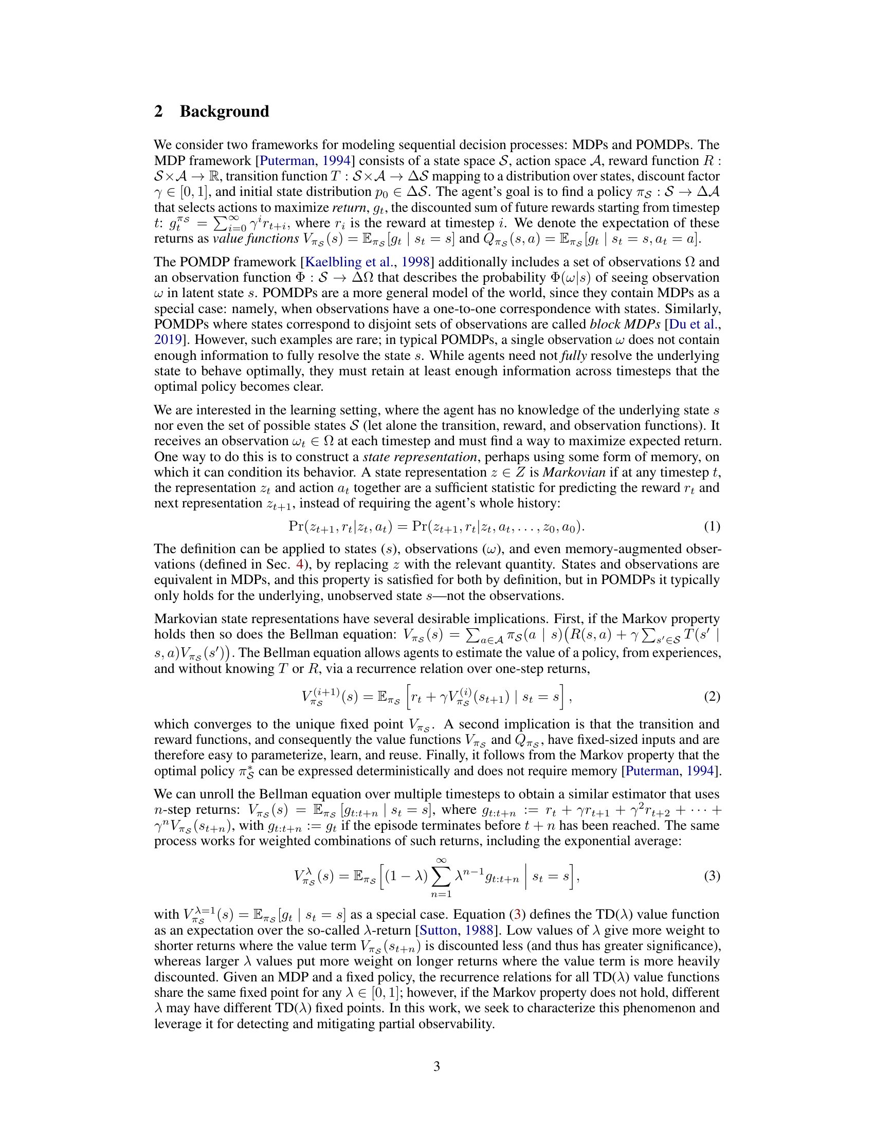
This figure shows a T-maze environment, a classic example of a partially observable Markov decision process (POMDP). The agent starts in one of two possible start states, represented by the color of the initial square (blue or red). The agent can only observe the color of the current square. The agent must reach the goal state (+1 reward) to obtain maximum reward. To do this, it needs to remember the color of the starting square. It must navigate the corridor and choose the correct path at the junction to reach the goal, highlighting the need for memory to overcome the partial observability.

This table shows the hyperparameters used in the experiments for the different algorithms. The hyperparameters were step size, lambda 1, lambda 2 (only for the A-discrepancy algorithm), and beta (only for the A-discrepancy algorithm). Each hyperparameter had a range of values which were tested.
In-depth insights#
Lambda Discrepancy#
The core concept of “Lambda Discrepancy” revolves around quantifying the deviation from the Markov assumption in sequential decision-making processes. It leverages Temporal Difference learning with varying lambda parameters (TD(λ)). TD(λ=0) implicitly assumes a Markov process, while TD(λ=1) is equivalent to Monte Carlo estimation and doesn’t make this assumption. The discrepancy between these value estimates serves as a powerful indicator of partial observability. A zero discrepancy suggests a Markovian system, whereas a non-zero discrepancy reveals the presence of hidden states or non-Markovian dynamics. This metric provides a principled approach to detect and mitigate partial observability, directly informing the need for memory mechanisms in reinforcement learning agents and guiding their design for improved performance in complex environments. Minimizing the lambda discrepancy becomes an effective auxiliary objective when training such agents, ensuring a more accurate state representation and leading to more robust policies.
POMDP Observability#
POMDP observability is a crucial aspect of reinforcement learning, as it directly impacts an agent’s ability to learn optimal policies. Partially observable Markov decision processes (POMDPs) pose significant challenges because the agent lacks complete state information, relying instead on noisy observations. This necessitates strategies to manage uncertainty and infer the hidden state. The paper explores methods for detecting and mitigating partial observability by introducing a metric called the lambda-discrepancy. This metric quantifies the difference between temporal difference (TD) estimates calculated using different values of lambda in TD(lambda), offering insights into the Markov property of the perceived state. The key idea is that a non-zero discrepancy highlights non-Markovianity, suggesting the need for memory or better state representation. The paper demonstrates this empirically and proposes an approach to integrate this into deep reinforcement learning. By minimizing the discrepancy as an auxiliary loss, the agent implicitly learns better state representations, leading to improved performance in complex POMDPs. The approach is valuable because it allows agents to learn effective state representations without explicit knowledge of the true underlying state space. This is a notable contribution towards making reinforcement learning more robust and applicable to real-world scenarios with inherent partial observability.
Memory Network#
A memory network, in the context of reinforcement learning, is a crucial component for handling partial observability. It acts as a mechanism to store and retrieve relevant information from past experiences, effectively augmenting the agent’s perception of the environment. The design and implementation of a memory network are critical; various architectures such as recurrent neural networks (RNNs) or specialized memory modules are used to store and process information. Effective memory networks are crucial for solving challenging partially observable Markov decision processes (POMDPs), improving decision-making quality. The choice of memory architecture often involves trade-offs between capacity, computational cost, and the ability to capture long-term dependencies. The learning process for memory networks typically includes mechanisms for optimizing the memory content itself based on the effectiveness of past decisions. Furthermore, the design often involves integrating the memory network with the agent’s value function and policy network creating a sophisticated and interconnected system for decision making and learning. The architecture must enable the agent to efficiently encode new experiences, retrieve relevant memories, and leverage that information for decision-making, potentially using attention mechanisms or other advanced techniques. Therefore, understanding how to design, implement and train a memory network is essential for addressing the challenges of partial observability in reinforcement learning, where the agent needs to remember relevant past information to make optimal decisions in the present.
Auxiliary Loss#
The concept of an auxiliary loss function is a powerful technique in deep learning that is particularly relevant to reinforcement learning problems, as discussed in the context of the research paper’s approach. An auxiliary loss is introduced to simultaneously address the challenge of partial observability. The primary goal of this strategy is to guide the learning process towards a more desirable state representation by explicitly penalizing discrepancies between multiple value function estimates produced by different temporal difference learning algorithms. The lambda discrepancy, which measures the extent of non-Markovianity in the observations, is minimized as an auxiliary loss. This forces the model to learn a better state representation and memory function, effectively mitigating the impact of partial observability. The effectiveness of incorporating this auxiliary loss is experimentally validated across various partially observable environments, demonstrating improved performance compared to baseline methods. The choice of an appropriate discrepancy metric and the weighting strategy in the auxiliary loss are crucial factors influencing the overall effectiveness of the approach. In essence, the auxiliary loss acts as a regularizer, shaping the learning dynamics to improve the quality of the learned state representation and ultimately the agent’s performance.
Future Work#
Future research directions stemming from this work on mitigating partial observability are plentiful. Extending the theoretical analysis of the lambda discrepancy to a broader class of POMDPs is crucial, as is exploring the boundary conditions where the metric fails to detect partial observability. Developing more sophisticated memory functions, possibly incorporating attention mechanisms or neural architectures beyond RNNs, could significantly improve performance in complex scenarios. Another promising area lies in combining the lambda discrepancy with other techniques for handling partial observability, such as state abstraction or belief-state representation, to create hybrid approaches that leverage the strengths of each method. Finally, rigorous empirical evaluations on a wider range of challenging POMDP benchmarks, including those with significant stochasticity and diverse reward structures, are necessary to fully assess the robustness and generality of the proposed approach. Investigating alternative methods for estimating the lambda discrepancy efficiently in deep RL settings is also warranted.
More visual insights#
More on figures
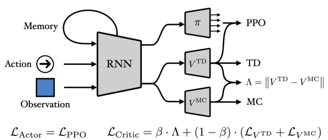
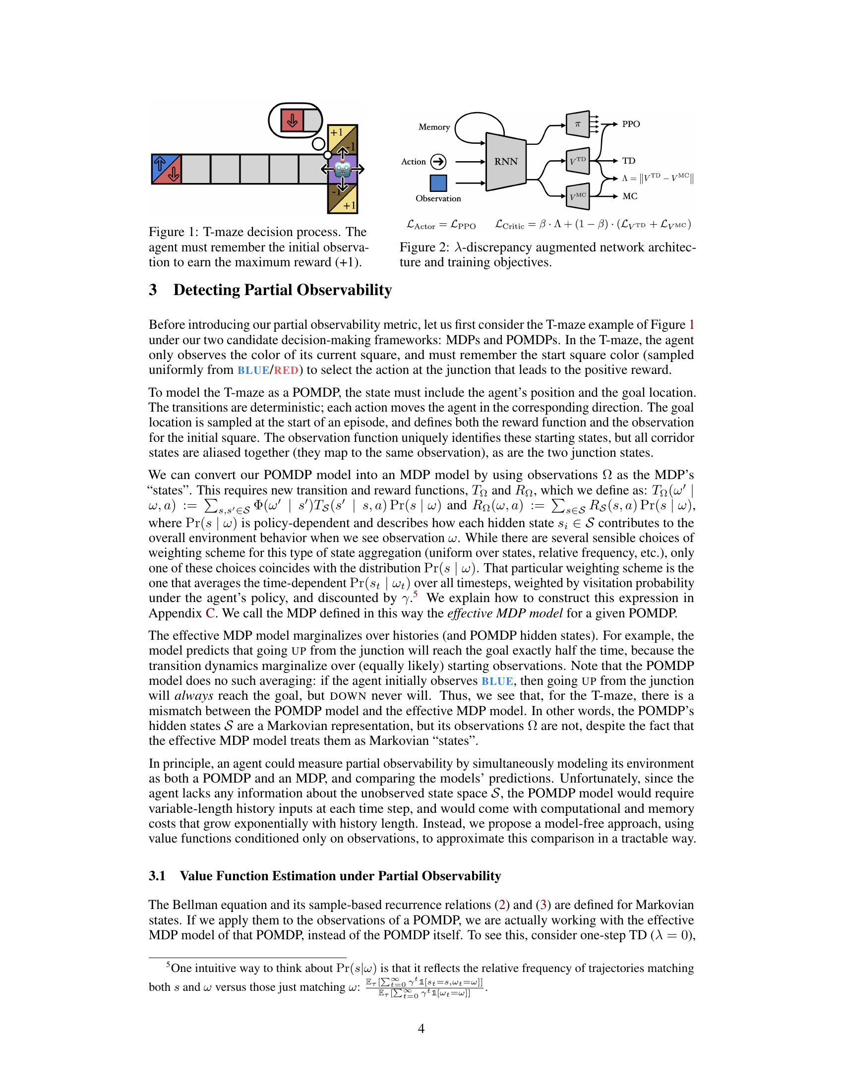
This figure illustrates the architecture of a neural network that uses the lambda discrepancy to mitigate partial observability. The network consists of an RNN (recurrent neural network) that takes as input the observation and action. The RNN’s output is fed into two separate value networks: one that estimates values using TD(λ) and another that estimates values using MC (Monte Carlo). The difference between the two value estimates is the lambda discrepancy, which is used as an auxiliary loss during training. The actor network is trained with the PPO algorithm, and its loss is a combination of the usual PPO loss and the lambda discrepancy loss. The critic network is trained to minimize the combination of the lambda discrepancy loss, and the TD(λ) and MC losses. The overall objective is to simultaneously learn a good state representation and a good policy.

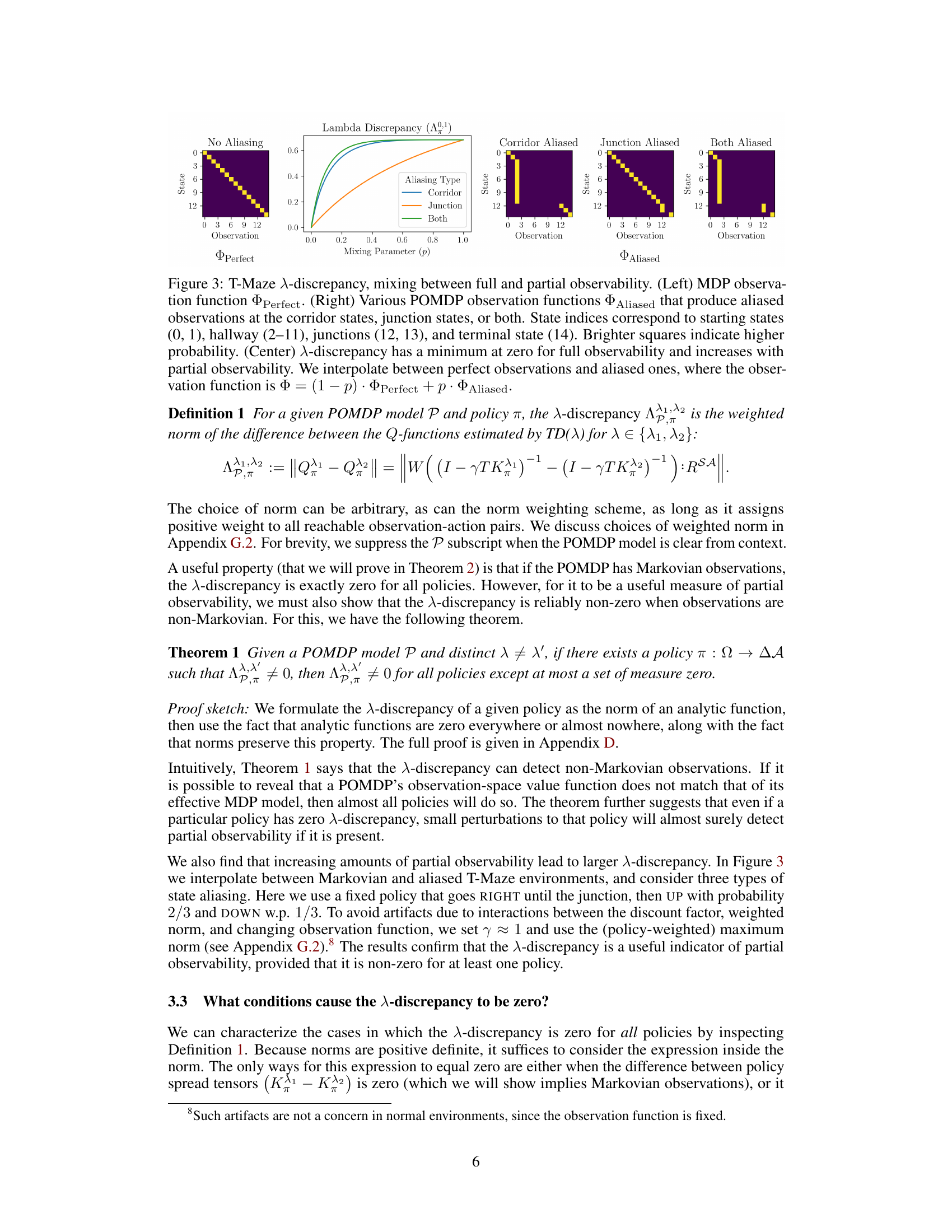
This figure shows how the lambda discrepancy changes depending on the level of partial observability in the T-maze environment. The left panel shows the observation function for a fully observable MDP (no aliasing). The right panels show observation functions for POMDPs with increasing levels of aliasing (corridor states aliased, junction states aliased, both aliased). The center panel plots the lambda discrepancy against a mixing parameter (p) which interpolates between the fully observable and partially observable observation functions. As expected, the lambda discrepancy increases with the degree of partial observability (i.e., aliasing).

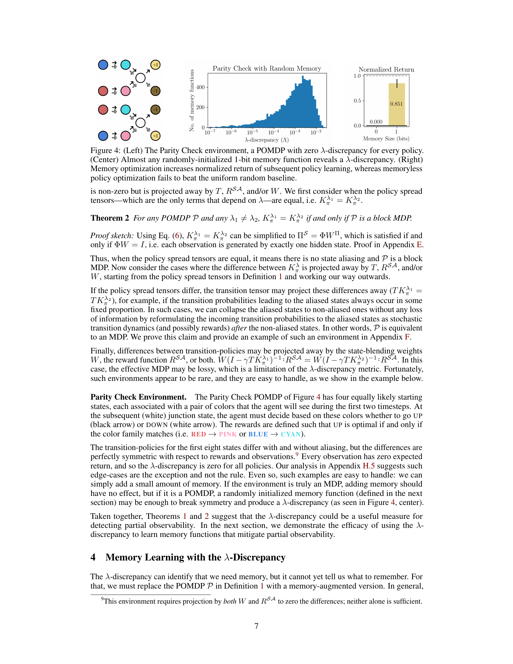
This figure shows three parts. The left part shows the Parity Check environment which is a POMDP with zero lambda discrepancy for any policy. The center part shows the distribution of lambda discrepancies for almost any randomly initialized 1-bit memory function in the Parity Check environment. The right part shows that minimizing lambda discrepancy increases the return of subsequent policy gradient learning, whereas memoryless policy optimization fails to beat the uniform random baseline.

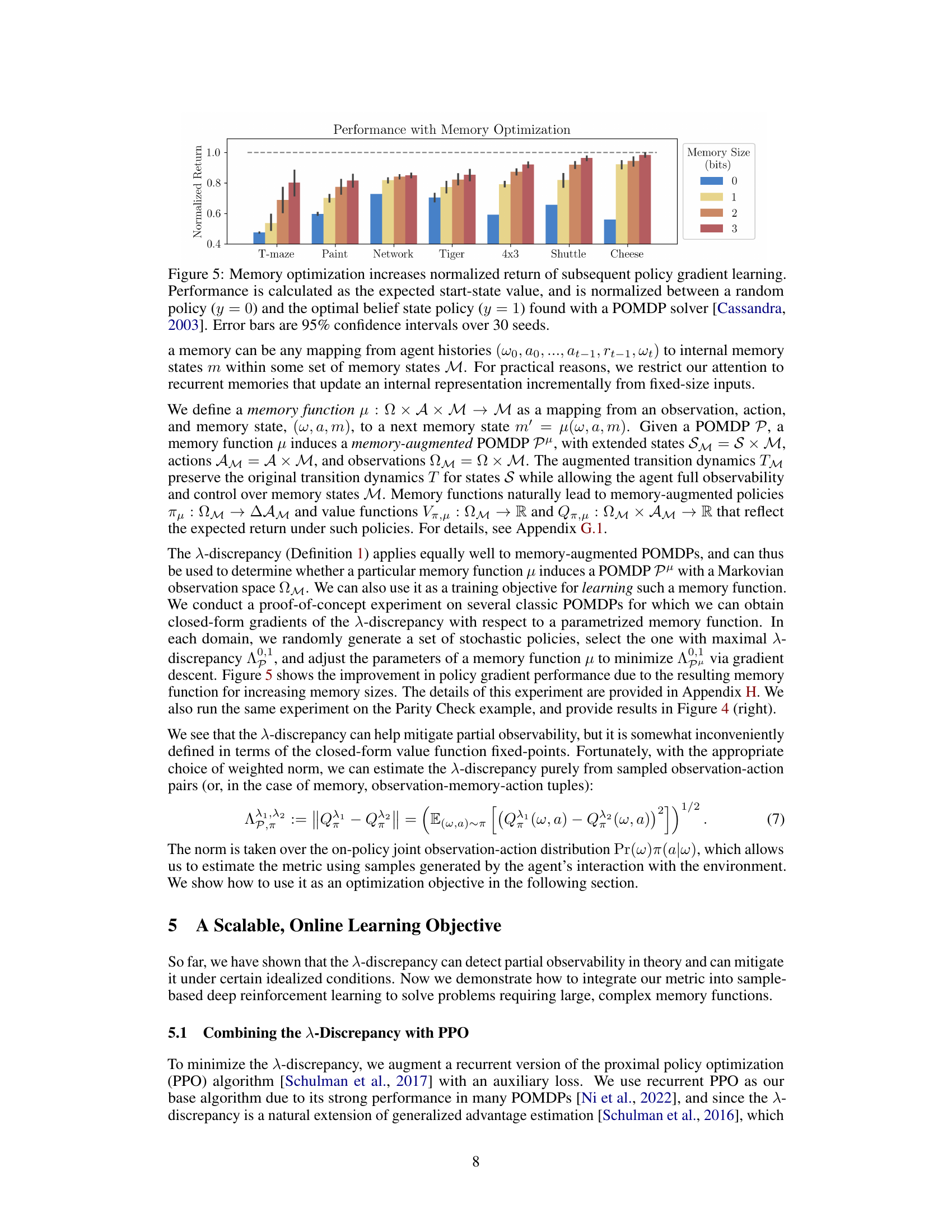
This figure shows the results of an experiment where a memory function was learned to improve the performance of a policy gradient algorithm on several POMDPs. The y-axis represents the normalized return, which is a measure of how much better the agent performs than a random policy. The x-axis shows different POMDPs. Each bar shows the results for a different memory size (0, 1, 2, or 3 bits). Error bars indicate the 95% confidence interval over 30 trials. The dashed line indicates the performance of an optimal policy.

This figure presents the experimental results of applying the λ-discrepancy auxiliary objective to four partially observable environments. The left panel shows the learning curves for the four environments. The right panel visualizes the agent’s memory in the Pac-Man environment, demonstrating the learned memory function’s effectiveness in improving performance.

This figure shows a POMDP with six states and an equivalent MDP with five states. The POMDP has non-Markovian observations because two distinct states produce the same observation. The key takeaway is that although the POMDP appears more complex, its behavior is identical to the simpler MDP; thus, the A-discrepancy is zero. This illustrates a situation where the A-discrepancy may not reliably identify partial observability.

This figure shows two versions of the Tiger POMDP. The left panel shows the original version, where the observation depends on both the state and the action. The right panel shows a modified version, where the observation only depends on the state. In the modified version, the states are colored to indicate the bias in the observation distribution. Purple states have an unbiased observation, while blue and red states have observations biased towards the left and right, respectively.

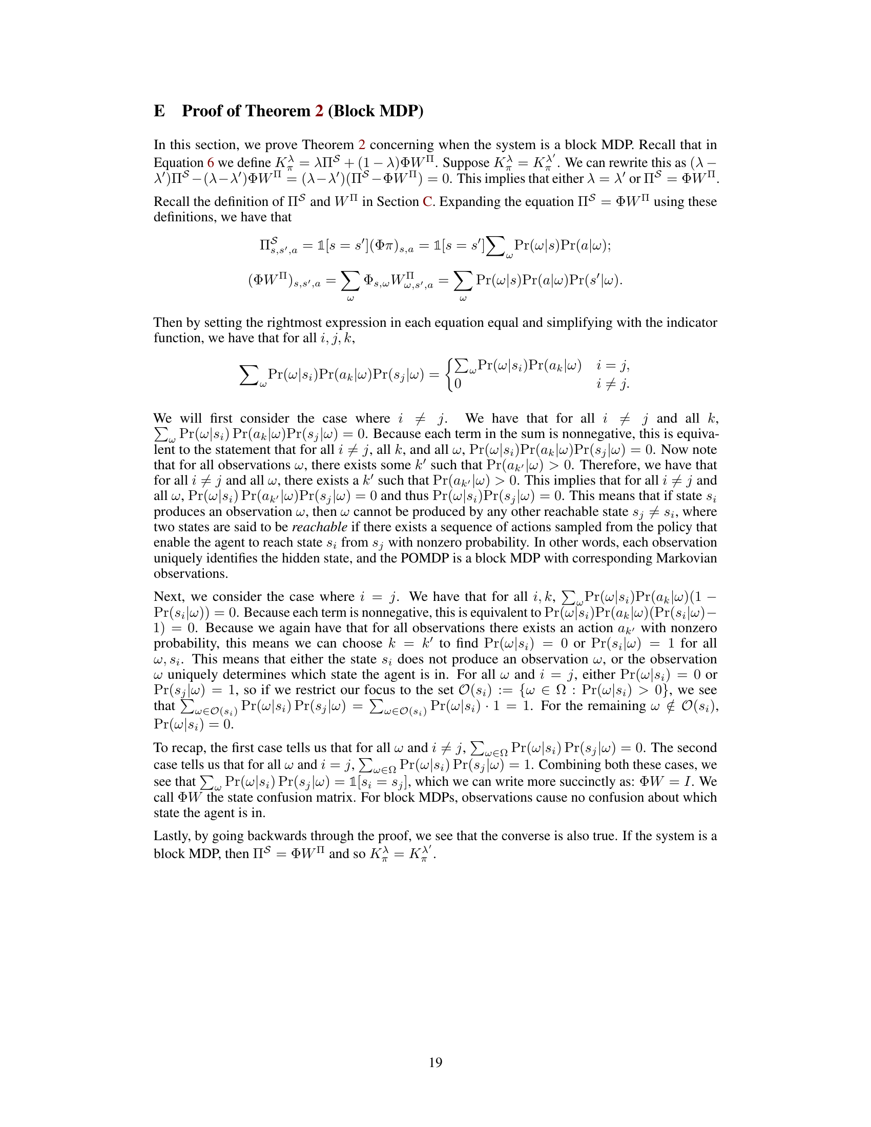
This figure shows that the Parity Check environment, which has zero λ-discrepancy for all policies, is a rare exception. Minor changes such as altering transition probabilities or initial state distribution result in non-zero λ-discrepancies for almost all policies, demonstrating the robustness of the λ-discrepancy metric in detecting partial observability.
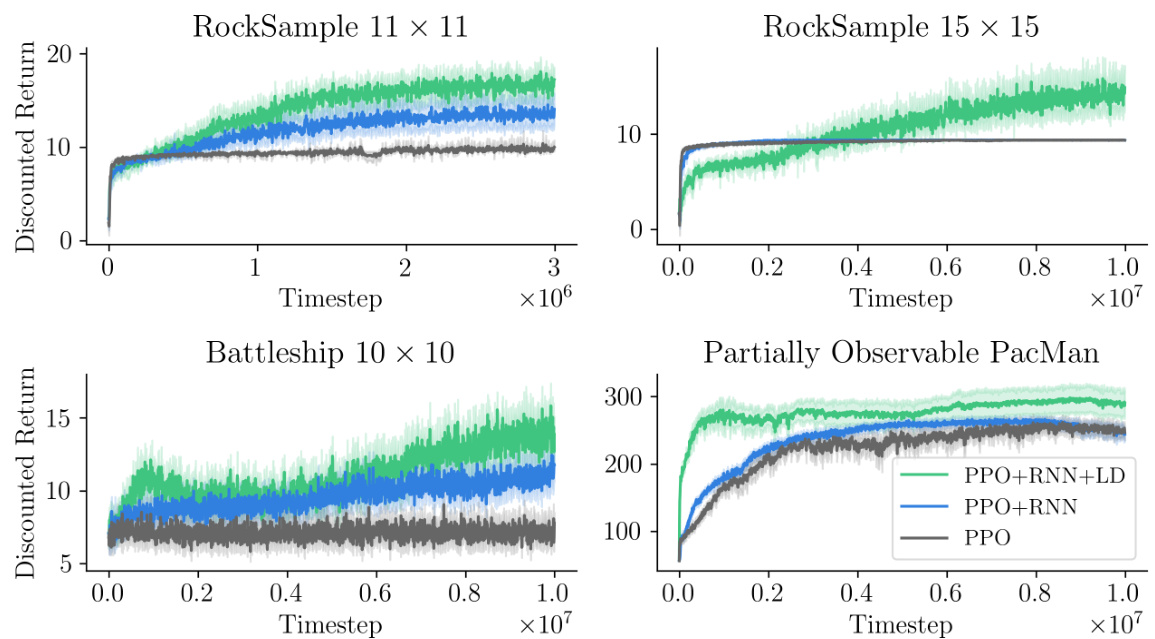
This figure presents the results of the proposed method on four challenging partially observable environments: RockSample (11x11), RockSample (15x15), Battleship (10x10), and Partially Observable Pac-Man. The left panel shows the learning curves for the three algorithms: PPO, PPO+RNN, and PPO+RNN+LD (λ-discrepancy). The PPO+RNN+LD algorithm consistently outperforms the other two algorithms in all environments. The right panel visualizes the agent’s memory for Partially Observable Pac-Man. The agent’s movement is shown in the middle panel. The bottom panel visualizes the memory of the recurrent neural network (RNN) without the auxiliary loss, while the top panel visualizes the memory with the auxiliary loss.
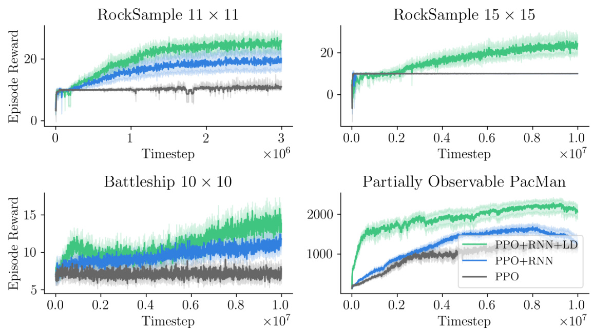
This figure presents the results of applying the proposed λ-discrepancy augmented recurrent PPO algorithm and compares it with recurrent PPO and memoryless PPO. The left panel shows learning curves across four different partially observable environments for the three algorithms, demonstrating that the auxiliary objective improves learning performance. The right panel provides a visualization of the agent’s memory in the partially observable Pac-Man environment, indicating how the agent’s memory helps in solving the partially observable navigation task. RNNs are shown to benefit from incorporating the λ-discrepancy as an auxiliary loss.
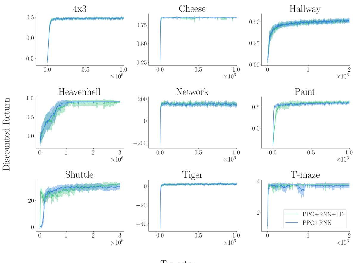
This figure shows the experimental results for four partially observable environments: RockSample (11x11), RockSample (15x15), Battleship (10x10), and Partially Observable Pac-Man. The left panel displays learning curves for each environment, comparing the performance of three algorithms: recurrent PPO (RNN), recurrent PPO with the λ-discrepancy auxiliary loss (RNN+LD), and memoryless PPO. The curves show that the algorithm with the λ-discrepancy auxiliary loss consistently outperforms the other two. The right panel shows a visualization of the agent’s memory in the Partially Observable Pac-Man environment. This visualization demonstrates that the agent is able to successfully maintain a representation of the environment and use it to make decisions.
More on tables

This table shows the best hyperparameters found for each of the four environments (Battleship, PacMan, RockSample (11, 11), and RockSample (15, 15)) across three different algorithms: A-discrepancy augmented recurrent PPO, recurrent PPO, and memoryless PPO. The hyperparameters were determined using a hyperparameter sweep across 5 random seeds, selecting the values that produced the maximum area under the learning curve (AUC). Each row represents an environment, and the columns list the step size, λ1, λ2 (used for calculating the λ-discrepancy), and β (the weighting factor for the λ-discrepancy loss).

This table shows the best hyperparameters found for each environment using five seeds and taking the maximum area under the learning curve (AUC). It lists the step size, lambda 1 value, lambda 2 value, and beta value for the A-discrepancy augmented recurrent PPO, recurrent PPO baseline, and memoryless PPO baseline. These values were used in the experiments described in the paper.

This table shows the hyperparameter settings used for the different environments in the experiments. It specifies the latent size of the neural networks and the entropy coefficient (CEnt) used in the training process. The entropy coefficient is a hyperparameter that controls the exploration-exploitation balance during training.
Full paper#


