↗ OpenReview ↗ NeurIPS Homepage ↗ Hugging Face ↗ Chat
TL;DR#
Deep learning model training often struggles with overfitting (too many training iterations) or underfitting (insufficient training data or iterations). Weight decay, a technique to prevent overfitting by penalizing large model weights, is widely used in both scenarios. However, its role remains unclear; classical theories primarily focus on its regularization effect, which is insufficient to explain its widespread use and efficacy in modern deep learning.
This paper investigated weight decay’s role in both over-training and under-training regimes. It reveals that weight decay’s true impact lies in altering training dynamics. In over-training, it stabilizes the loss function, leading to more stable training with larger learning rates. In under-training, it helps balance bias and variance tradeoff for better model accuracy. This work provides a unifying perspective on weight decay’s role, irrespective of training regime, and suggests that it isn’t primarily a regularizer but a tool to improve optimization dynamics.
Key Takeaways#
Why does it matter?#
This paper is crucial because it challenges the conventional understanding of weight decay in deep learning. By offering nuanced explanations for its effectiveness in different training scenarios, it guides researchers towards more effective model training, particularly for large language models and image recognition. The findings open up new avenues for optimization techniques and improve our understanding of the complex dynamics of deep learning training.
Visual Insights#
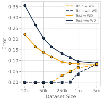
This figure shows the test error rate plotted against the dataset size for a ResNet18 model trained on the CIFAR-10-5m dataset. Two training scenarios are compared: one with weight decay and one without. The results demonstrate that weight decay improves the test error rate across a range of dataset sizes, regardless of whether the model is in an over-training or under-training regime.

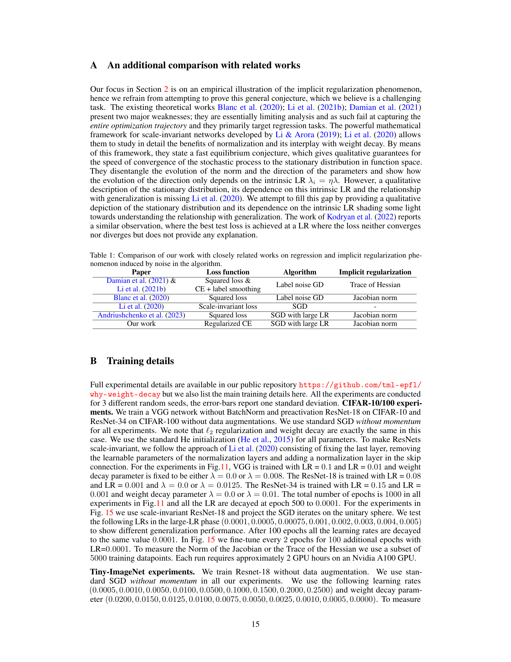
This table compares the author’s work to other closely related works on regression and implicit regularization. It highlights the differences in loss functions, algorithms, and the type of implicit regularization achieved. The comparison helps to situate the author’s contributions within the existing literature on the topic.
In-depth insights#
Weight Decay’s Dual Roles#
Weight decay, a seemingly simple regularization technique, exhibits surprising complexity. The paper reveals its dual roles in modern deep learning, depending on the training regime. In over-parametrized models trained for many epochs, weight decay primarily alters optimization dynamics. It stabilizes the loss function, preventing unbounded growth of the weight norm and thus enabling the implicit regularization inherent in SGD with large learning rates. However, in under-trained models, such as LLMs trained with a single epoch, weight decay acts differently, essentially modifying the effective learning rate and thus influencing the bias-variance tradeoff, leading to better training stability and lower loss. This dual nature highlights the nuanced impact of weight decay, underscoring the need to move beyond simple regularization interpretations and consider its influence on optimization dynamics.
SGD Noise & Generalization#
The interplay between SGD noise and generalization is a crucial aspect of deep learning. SGD’s inherent stochasticity, while seemingly a drawback, introduces beneficial noise into the optimization process. This noise, far from being detrimental, acts as a form of implicit regularization. It prevents the model from converging to sharp minima in the loss landscape, which are often associated with overfitting. Instead, the noise encourages the model to find flatter minima that generalize better to unseen data. Weight decay plays a significant role in modulating this effect by controlling the scale of the noise. With large learning rates, weight decay balances the bias-variance tradeoff, leading to improved generalization performance and stable training dynamics, especially in the presence of limited training data or computational resources. Understanding this noise-driven optimization is vital for improving deep learning models’ generalization ability and robustness.
Implicit Regularization#
Implicit regularization, a phenomenon where the training dynamics of a model implicitly leads to a preference for certain solutions over others, is a crucial concept in deep learning. It’s not explicitly programmed, but emerges from the interplay of the optimization algorithm (like SGD) and the model’s architecture. Understanding implicit regularization is key to explaining the generalization ability of deep learning models, especially in scenarios where the models are over-parameterized, or trained with large amounts of data. Research suggests that the use of weight decay, a seemingly simple regularization technique, interacts with the implicit regularization of SGD in complex ways, leading to improved generalization. While still an active area of research, the concept of implicit regularization provides a deeper understanding of the effectiveness of deep learning models, paving the way for future advancements.
Bias-Variance Tradeoff#
The bias-variance tradeoff is a central concept in machine learning, representing the tension between model complexity and its ability to generalize to unseen data. High bias implies a model is too simplistic, failing to capture the underlying patterns in the data, leading to underfitting. High variance, on the other hand, signifies an overly complex model that is highly sensitive to noise and training data specifics, resulting in overfitting. Finding the optimal balance is crucial; a model with low bias and low variance achieves the best generalization performance, accurately predicting outcomes on new, unseen data. Techniques like regularization, cross-validation, and choosing appropriate model complexity help manage this tradeoff, ultimately leading to more robust and reliable machine learning models. The choice of model architecture and hyperparameters directly influence this tradeoff, highlighting the need for careful experimentation and selection to strike the right balance between model fit and generalization.
Bfloat16 Stability#
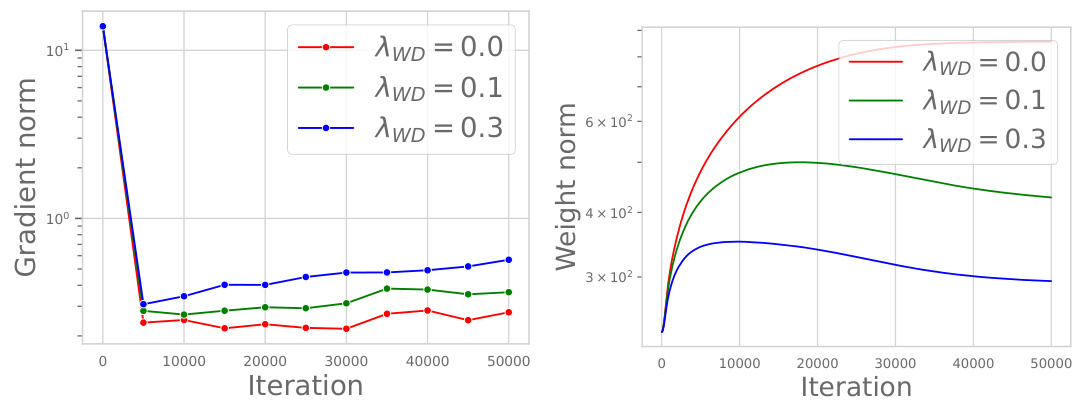
The use of bfloat16, a reduced-precision floating-point format, presents a trade-off between computational efficiency and numerical stability. While offering significant speedups, bfloat16’s limited precision can lead to training instability, especially in large language models. Weight decay plays a crucial role in mitigating this instability, allowing for stable training even with the reduced precision of bfloat16. This suggests that weight decay’s impact extends beyond regularization, influencing the optimization dynamics in a way that enhances robustness to numerical errors inherent in bfloat16 computations. The improved stability, however, appears closely tied to specific hyperparameter choices, implying that successful utilization requires careful tuning and possibly a dependency on the specific model architecture. Further research is needed to fully understand this interaction between weight decay, bfloat16 precision, and the underlying optimization dynamics. The practical benefit of achieving stable training with bfloat16 is substantial, considering its implications for computational cost and accessibility in large-scale model training.
More visual insights#
More on figures

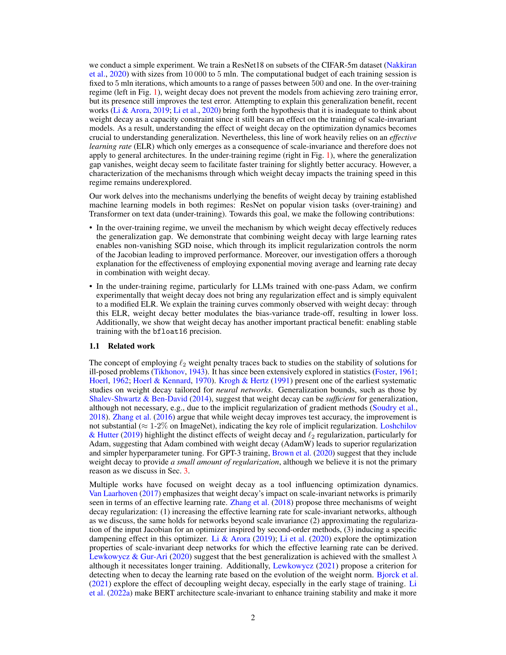
This figure compares the performance of ResNet18 trained on CIFAR-10 and TinyImageNet with and without weight decay, using both small and large learning rates. It includes plots showing test error, training cross-entropy, L2 norm of parameters, and the effect of exponential moving average (EMA). The results highlight the impact of weight decay on optimization dynamics, showing that weight decay modifies the training dynamics in a beneficial way even when the models fully memorize the training data.

This heatmap visualizes the test error and Frobenius norm of the Jacobian (a measure of model complexity) for a ResNet18 model trained on the Tiny-ImageNet dataset. The heatmap shows how these metrics vary across different combinations of the learning rate (η) and weight decay parameter (λ). The results are obtained using the Exponential Moving Average (EMA) of the model parameters, offering insight into the model’s performance and generalization behavior under different optimization strategies.

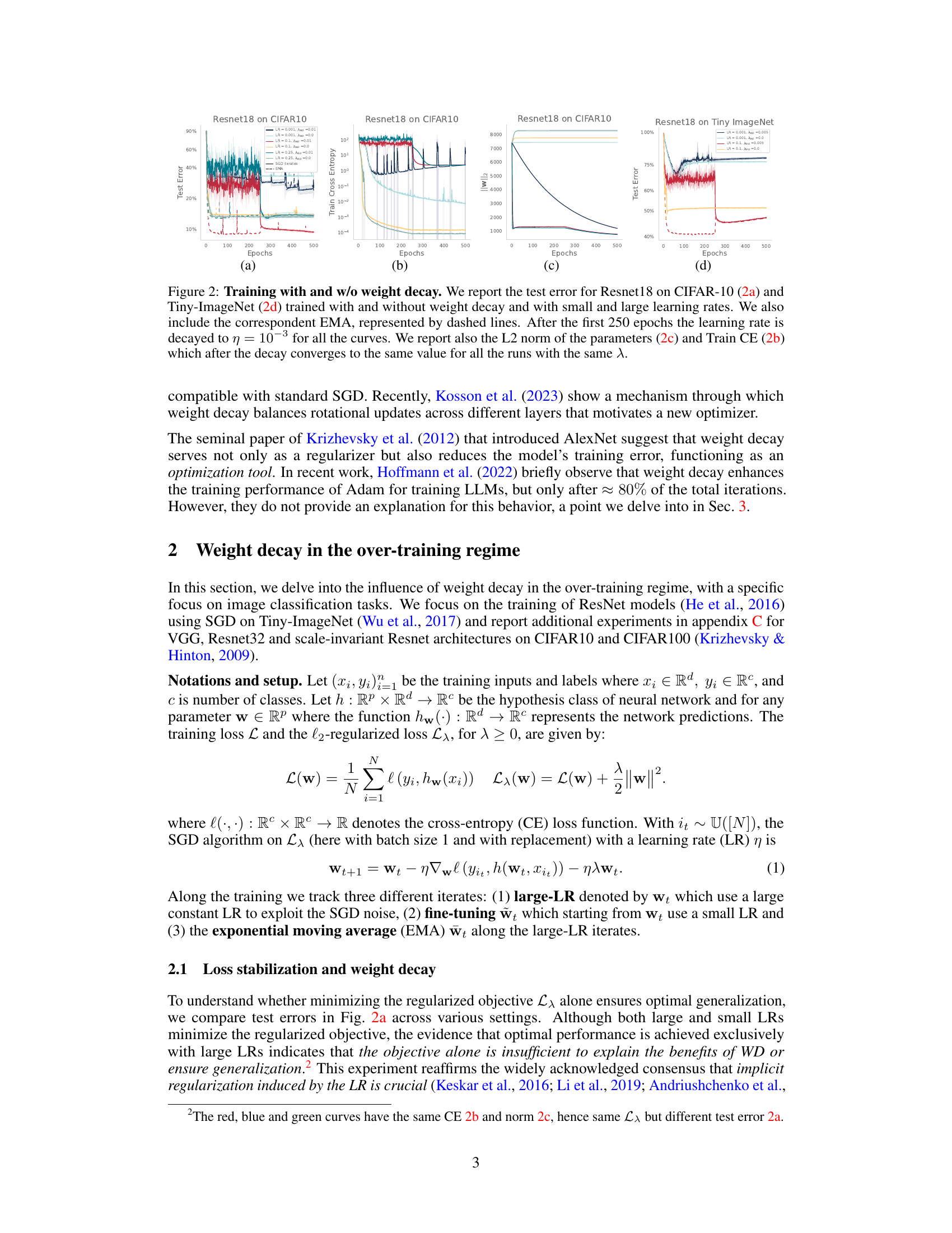
This figure shows the results of training ResNet18 on the Tiny-ImageNet dataset for 200 epochs with various learning rates (η) and weight decay parameters (λ). Panel (a) demonstrates that the scale of the noise (ση,λ), a crucial factor in the implicit regularization mechanism, increases monotonically with both the training loss and the product of η and λ. Panel (b) shows a similar monotonic relationship between ση,λ and the product of η and λ. However, panel (c) reveals that there’s an optimal value for the product ηλ that minimizes the test error. Finally, panel (d) shows a consistently decreasing Jacobian norm (||J||F) with increasing ηλ, suggesting that over-regularization occurs beyond the optimal ηλ value. The figure strongly suggests an optimal balance between noise and regularization for best generalization performance.

This figure shows the effect of weight decay on the test error and training dynamics of ResNet18 on CIFAR-10 and TinyImageNet. It compares models trained with and without weight decay, using both small and large learning rates. The plots illustrate test error, training cross-entropy, L2 norm of the parameters, and the effect of exponential moving average (EMA). The learning rate is decayed after 250 epochs.
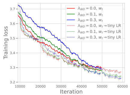
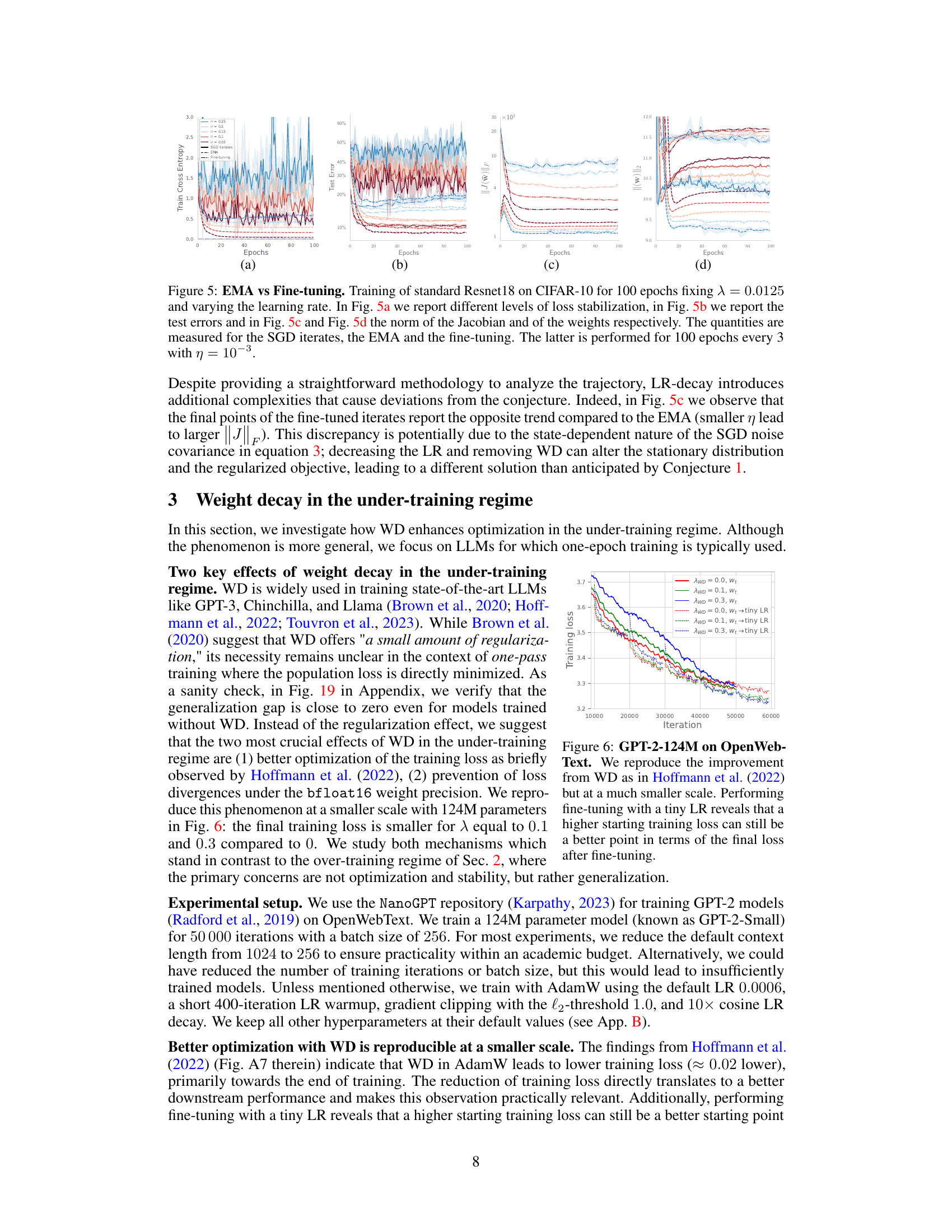
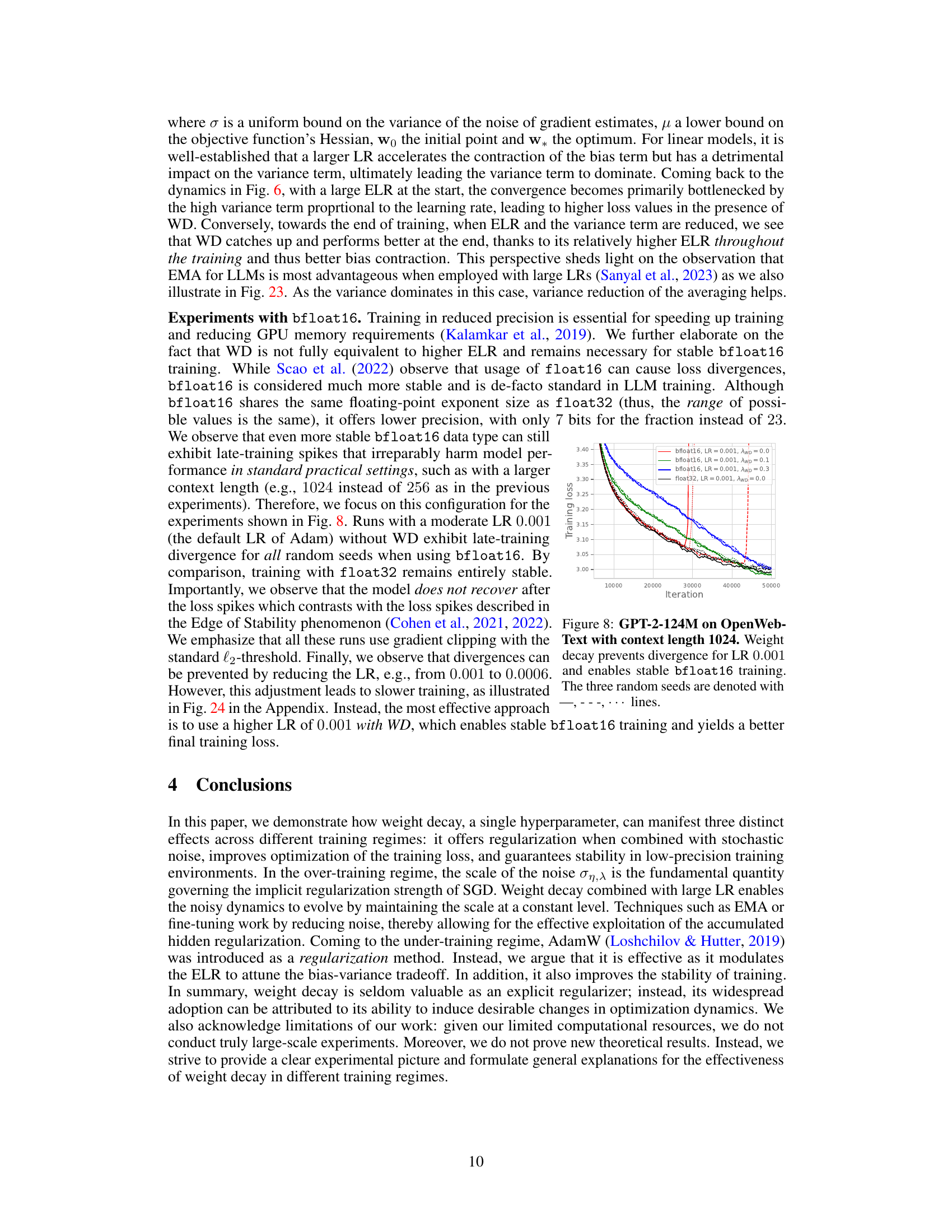
This figure shows the training loss curves for a GPT-2 language model with 124M parameters trained on the OpenWebText dataset. Multiple curves are presented, each representing a different weight decay (λwd) value (0.0, 0.1, and 0.3). For each weight decay value, two curves are shown: one for training with the standard learning rate schedule, and another after fine-tuning with a very small learning rate. The results indicate that using weight decay can lead to a lower training loss, even if the initial training loss is higher than when no weight decay is used. The authors replicate findings from prior work (Hoffmann et al., 2022) using a smaller scale model for validation.

This figure demonstrates that the effective learning rate (ηt/||wt||2) is a key factor influencing the training dynamics of large language models. The left panel shows the effective learning rate for different models trained with varying weight decay (λ). The middle panel shows a learning rate schedule that mimics the effective learning rate of the models with weight decay. The right panel compares the training loss curves, showing that matching the effective learning rate is enough to reproduce the dynamics but only when higher precision (float32) is used instead of bfloat16.

This figure shows the training loss curves for a GPT-2 language model with 124M parameters, trained on the OpenWebText dataset. Multiple curves are shown, representing different weight decay (λ_{wd}) hyperparameter values (0.0, 0.1, and 0.3). The key takeaway is that while weight decay doesn’t prevent the model from achieving zero training error, its presence still improves the test error (generalization) as shown by Hoffmann et al. (2022). The experiment also demonstrates that a higher starting training loss, facilitated by weight decay, can lead to a lower final training loss after a fine-tuning phase with a smaller learning rate. This highlights that weight decay’s role isn’t solely about regularization, but also about affecting the optimization dynamics in a favorable way.
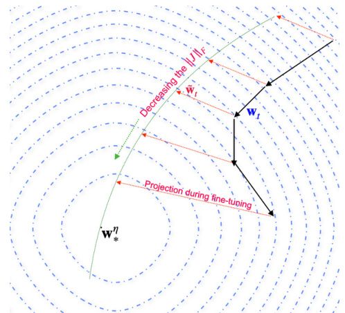
This figure provides a visual illustration of the fine-tuning phase. The green curve represents the trajectory of the SGD iterates in the large-LR phase. As the training proceeds, the trajectory moves towards a solution, represented by the star (*). The black lines indicate the projections of SGD iterates onto the manifolds with the same CE values, which are concentric circles around the solution. The red lines show the distances between SGD iterates and the projections onto these circles. The figure highlights the decreasing Jacobian norm in the fine-tuning phase.

This figure shows heatmaps of the test error and Frobenius norm of the Jacobian for an EMA (Exponential Moving Average) across various combinations of learning rate (η) and weight decay (λ) for a ResNet18 model trained on the Tiny-ImageNet dataset. The heatmaps visualize the relationship between these hyperparameters and model performance, illustrating how the optimal test error is not achieved by a single combination of η and λ but rather along a contour where their product η × λ is approximately constant. The Jacobian norm shows a consistently decreasing trend as the product ηλ increases.

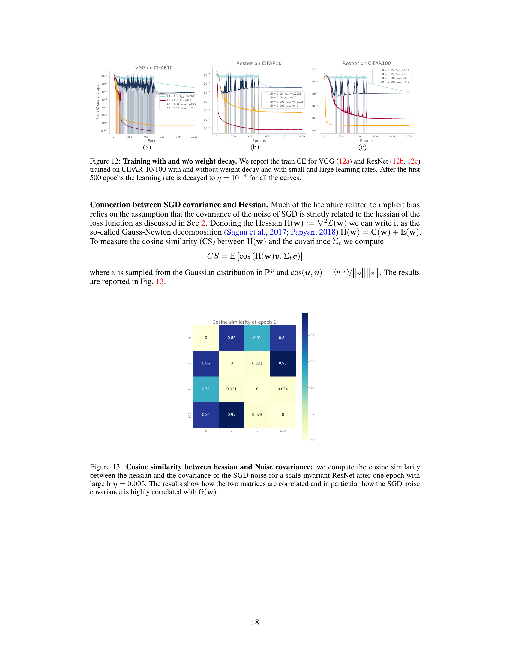
The figure shows the test error for VGG and ResNet models trained on CIFAR-10 and CIFAR-100 datasets with and without weight decay. The models were trained with both small and large learning rates. After 500 epochs, the learning rate was decayed for all curves. The results illustrate the impact of weight decay and learning rate on model performance.

This figure compares the training cross-entropy (CE) loss curves for VGG and ResNet models trained on CIFAR-10 and CIFAR-100 datasets, respectively. The models are trained with and without weight decay (WD), and with both small and large learning rates. The learning rate is decayed after 500 epochs. The figure illustrates how weight decay affects the training dynamics, specifically the convergence of the training loss.

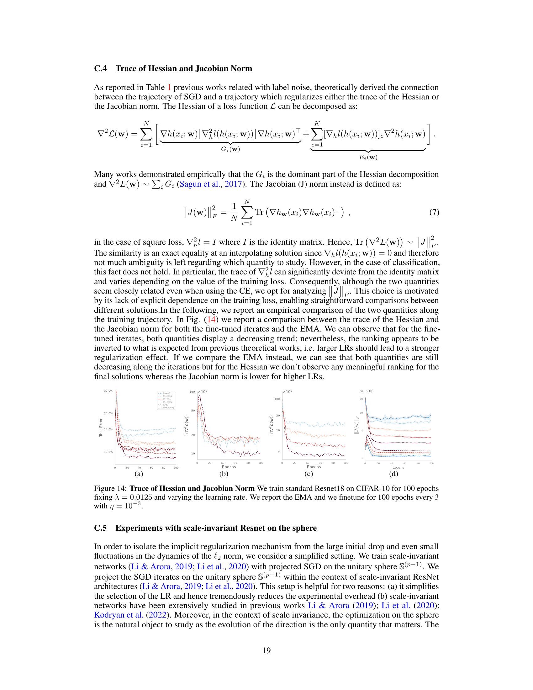
This figure shows the cosine similarity between the Hessian and the noise covariance of SGD for a scale-invariant ResNet after one epoch with a large learning rate. The high correlation between the noise covariance and the Gauss-Newton component (G) of the Hessian supports the paper’s argument that SGD’s implicit regularization is driven by noise.

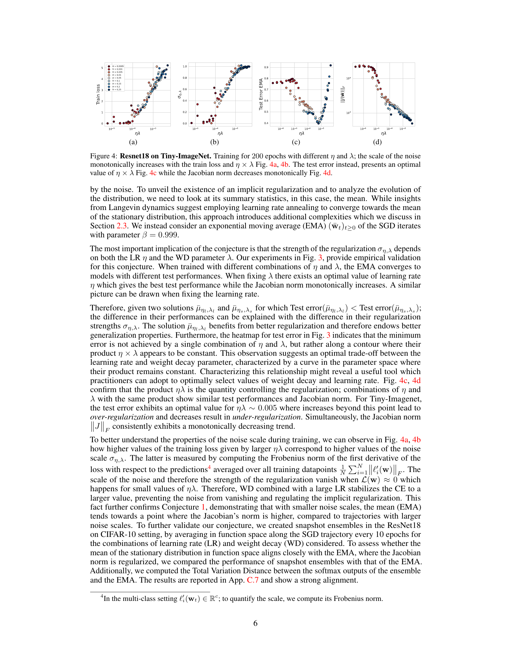
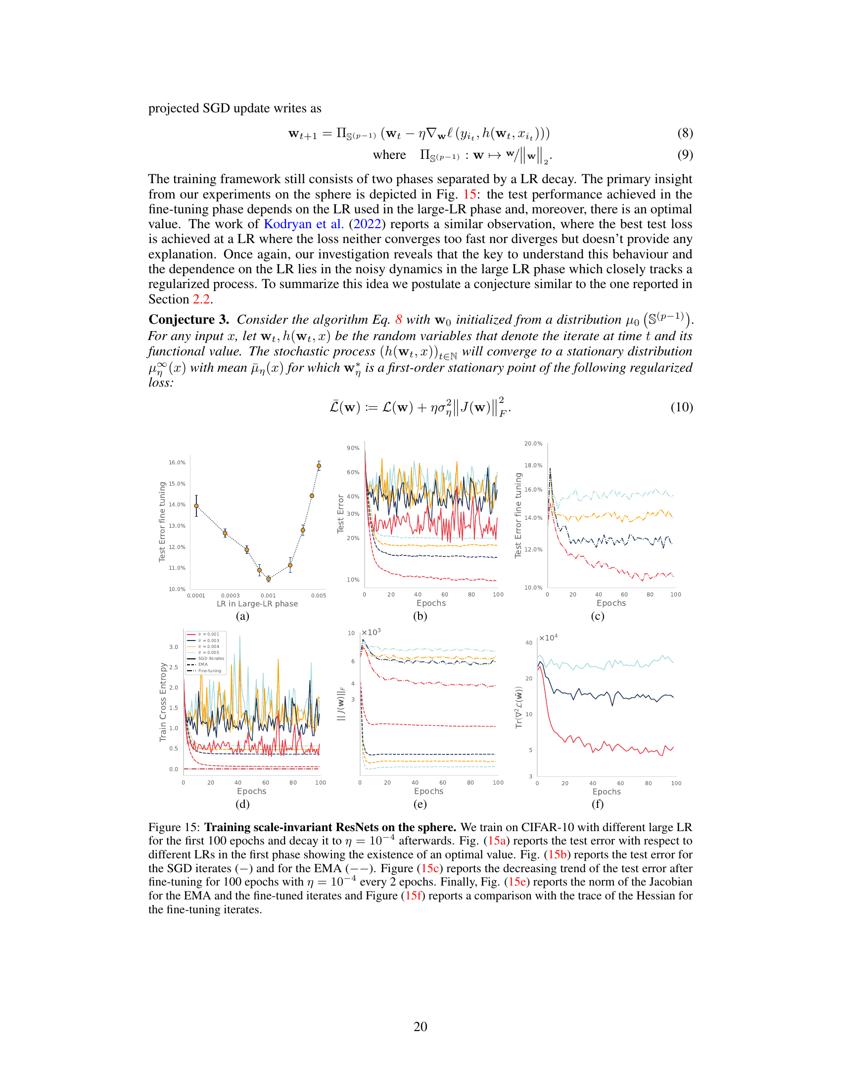
This figure compares the performance of EMA and fine-tuning methods for ResNet18 trained on CIFAR-10. It shows the training loss stabilization, test errors, Jacobian norm, and weight norm for different learning rates. The results indicate that both EMA and fine-tuning improve performance, but EMA is slightly more efficient.

This figure compares the training dynamics of Resnet18 on CIFAR-10 using EMA (Exponential Moving Average) and fine-tuning methods. It shows the training loss, test error, Jacobian norm, and weight norm for different learning rates with a fixed weight decay of 0.0125. Fine-tuning involves decaying the learning rate after a certain number of epochs. The results illustrate the interplay between the learning rate, weight decay, and the optimization dynamics, and how EMA and fine-tuning influence the performance of the model.

This figure shows a heatmap visualizing the test error and Frobenius norm of the Jacobian for an Exponential Moving Average (EMA) of the parameters. The heatmap covers various combinations of learning rate (η) and weight decay (λ). The goal is to illustrate the interplay between these hyperparameters in influencing the model’s generalization performance, as measured by the test error, and the complexity of the model as measured by the Jacobian norm.
This figure shows a heatmap visualizing the test error and Frobenius norm of the Jacobian for an Exponential Moving Average (EMA) of the model’s weights. The heatmap explores various combinations of the learning rate (η) and weight decay parameter (λ) during the training of a ResNet18 model on the Tiny-ImageNet dataset. The results illustrate the interplay between these hyperparameters in achieving optimal generalization performance and controlling the norm of the learned model’s Jacobian.
This figure shows a heatmap visualizing the test error and Frobenius norm of the Jacobian for an Exponential Moving Average (EMA) of the SGD iterates. The heatmap is generated by varying the learning rate (η) and weight decay parameter (λ) across a range of values. The results illustrate the interplay between these two hyperparameters in determining both the generalization performance (test error) and the model’s complexity (Jacobian norm).
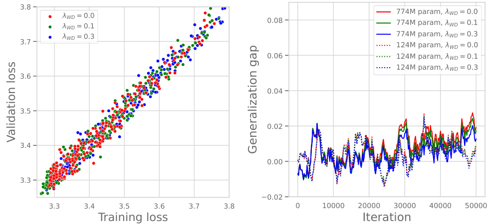
This figure shows the relationship between training loss and validation loss for GPT-2 language models with varying numbers of parameters (124M and 774M) and different weight decay hyperparameters (λ). The left panel demonstrates a strong correlation between training and validation loss, irrespective of the weight decay value. The right panel illustrates that the generalization gap (the difference between training and validation loss) remains consistently near zero across all experimental settings, suggesting that weight decay doesn’t significantly impact the model’s ability to generalize.
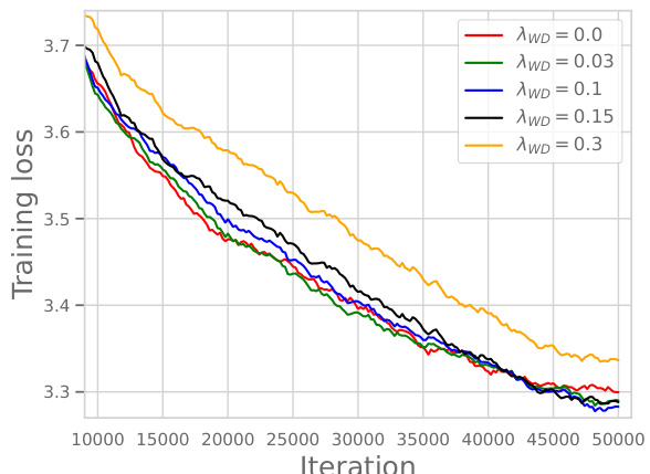
This figure shows the training loss curves for a GPT-2-124M language model trained on the OpenWebText dataset with different weight decay (λwd) values. It demonstrates that while weight decay doesn’t prevent the model from achieving zero training error, it improves the final training loss, especially when combined with a small learning rate during fine-tuning. This highlights the impact of weight decay on optimization dynamics, specifically improving training loss in the under-training regime where only a single pass through the data is done.

This figure shows the training loss curves for a GPT-2-124M language model trained on the OpenWebText dataset with different weight decay values (λ_{WD}). It demonstrates that even though weight decay does not prevent the models from achieving zero training error, its presence still leads to a lower training loss and ultimately better generalization (not shown but mentioned in the paper). The effect is more pronounced at the end of training, but a higher initial training loss with weight decay results in a better final loss after fine-tuning with a smaller learning rate.
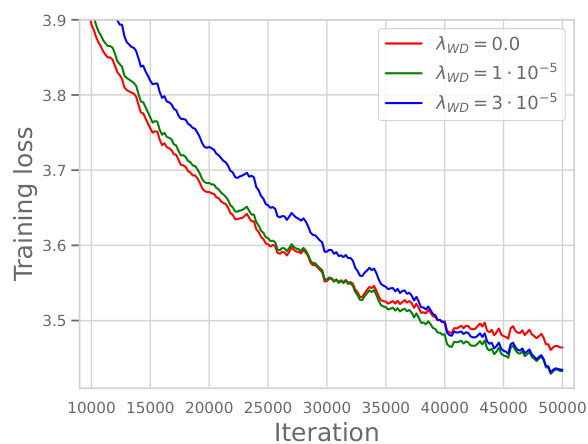
This figure shows the training loss curves for a GPT-2-124M language model trained on the OpenWebText dataset using AdamW optimizer with different weight decay values (λWD). The experiment demonstrates that weight decay (WD) leads to lower training loss, even when employing a small learning rate during the fine-tuning phase. This suggests that WD primarily affects the optimization dynamics rather than explicit regularization, especially in the under-training regime. The results confirm Hoffmann et al.’s (2022) findings at a smaller scale.

This figure compares the test error, training cross-entropy, and L2 norm of the parameters for ResNet18 trained on CIFAR-10 and TinyImageNet with and without weight decay, using both small and large learning rates. The effect of exponential moving average (EMA) is also shown. The learning rate is decayed after 250 epochs. The results illustrate the impact of weight decay on model generalization and optimization dynamics in different settings.

This figure shows the results of training ResNet18 on the Tiny-ImageNet dataset for 200 epochs using different learning rates (η) and weight decay parameters (λ). The plots demonstrate the relationship between the training loss, the scale of the noise (ση,λ), the test error, and the Frobenius norm of the Jacobian (||J(W)||F). Specifically, it highlights that while the noise scale increases monotonically with both training loss and the product of learning rate and weight decay (ηλ), the test error exhibits an optimal value of ηλ. The Jacobian norm, conversely, decreases monotonically.

This figure shows the results of training ResNet18 on the Tiny-ImageNet dataset for 200 epochs with different learning rates (η) and weight decay parameters (λ). It demonstrates that the scale of the noise in the optimization process increases monotonically with both the training loss and the product of η and λ. However, the test error shows an optimal value for the product ηλ, indicating a trade-off between learning rate and weight decay. Finally, the figure shows that the Jacobian norm of the model decreases monotonically with increasing ηλ.
This figure shows the results of experiments on training ResNet18 on the Tiny-ImageNet dataset for 200 epochs using different learning rates (η) and weight decay parameters (λ). It demonstrates the relationship between these hyperparameters, the training loss, test error, and Jacobian norm. Notably, the scale of the noise (a key factor influencing generalization) increases monotonically with both the training loss and the product of learning rate and weight decay (ηλ). However, the test error achieves an optimal value at a specific ηλ, while the Jacobian norm decreases consistently, suggesting that there exists an optimal balance between the noise scale and the norm of the Jacobian for best generalization.
More on tables

This table presents the test error for both snapshot ensembles and exponential moving averages (EMA) across various learning rates (LR) and weight decay (WD) values. It allows for a comparison of the two methods’ performance under different hyperparameter settings. The results are used to support the conjecture proposed in the paper regarding the implicit regularization mechanism.

This table presents the Total Variation Distance (TVD) between the softmax outputs of the snapshot ensemble and the exponential moving average (EMA) for various combinations of learning rates (LR) and weight decay (WD) parameters. The TVD quantifies the difference in probability distributions between the ensemble and EMA predictions. Lower TVD values indicate a stronger agreement between the two methods, thus supporting the claim that the EMA closely tracks the behavior of the ensemble and represents a good approximation of the stationary distribution during training.
Full paper#

