Optimal Top-Two Method for Best Arm Identification and Fluid Analysis

↗ OpenReview ↗ NeurIPS Homepage ↗ Chat

TL;DR

#

Key Takeaways

#

Why does it matter?

#

This paper is crucial for researchers in best arm identification due to its novel optimal top-two algorithm. It offers significant improvements in efficiency and computational cost compared to existing methods, impacting fields like healthcare and recommendation systems that rely on efficient BAI. The use of fluid dynamics and the implicit function theorem provides a new analytical approach for solving BAI problems, opening new avenues for research in related areas.

Visual Insights

#

The figure shows the evolution of the normalized indexes of the suboptimal arms in a 4-armed Gaussian bandit with unit variance and mean vector μ = [10, 8, 7, 6.5] for the AT2 algorithm (without stopping rule). The plot demonstrates how the indexes of suboptimal arms tend to converge once they come close to each other during the course of the algorithm. This convergence behavior is a key characteristic of the fluid dynamics underlying the AT2 algorithm and is important for its asymptotic optimality.

The table shows the average runtime and standard deviation of four algorithms (AT2, IAT2, TCB, and ITCB) for a Gaussian bandit with specified parameters. The runtime was averaged over 100,000 independent runs of each algorithm. The experiment is labeled as Experiment 6 in the paper.

In-depth insights

#

Fluid Model’s Role

#

The paper leverages a ‘fluid model’ to analyze the asymptotic behavior of their proposed best arm identification algorithm. This model simplifies the complex stochastic dynamics of the algorithm by approximating the discrete allocation of samples to a continuous process governed by ordinary differential equations (ODEs). The fluid model is crucial for understanding the algorithm’s convergence to optimality. It provides an intuitive and mathematically tractable way to describe how the allocation proportions of samples to different arms evolve, ultimately approaching the theoretical optimum as the number of samples increases. By analyzing the ODEs, the authors gain insights into the algorithm’s asymptotic performance, providing strong support for its optimality claims. This approach significantly simplifies analysis and offers a powerful framework to study complex sequential decision-making problems. The fluid model’s elegance lies in its ability to bridge the gap between the discrete, stochastic reality of the algorithm and a continuous, deterministic approximation, making it a powerful tool for understanding the long-term behavior of the algorithm.

AT2 Algorithm

#

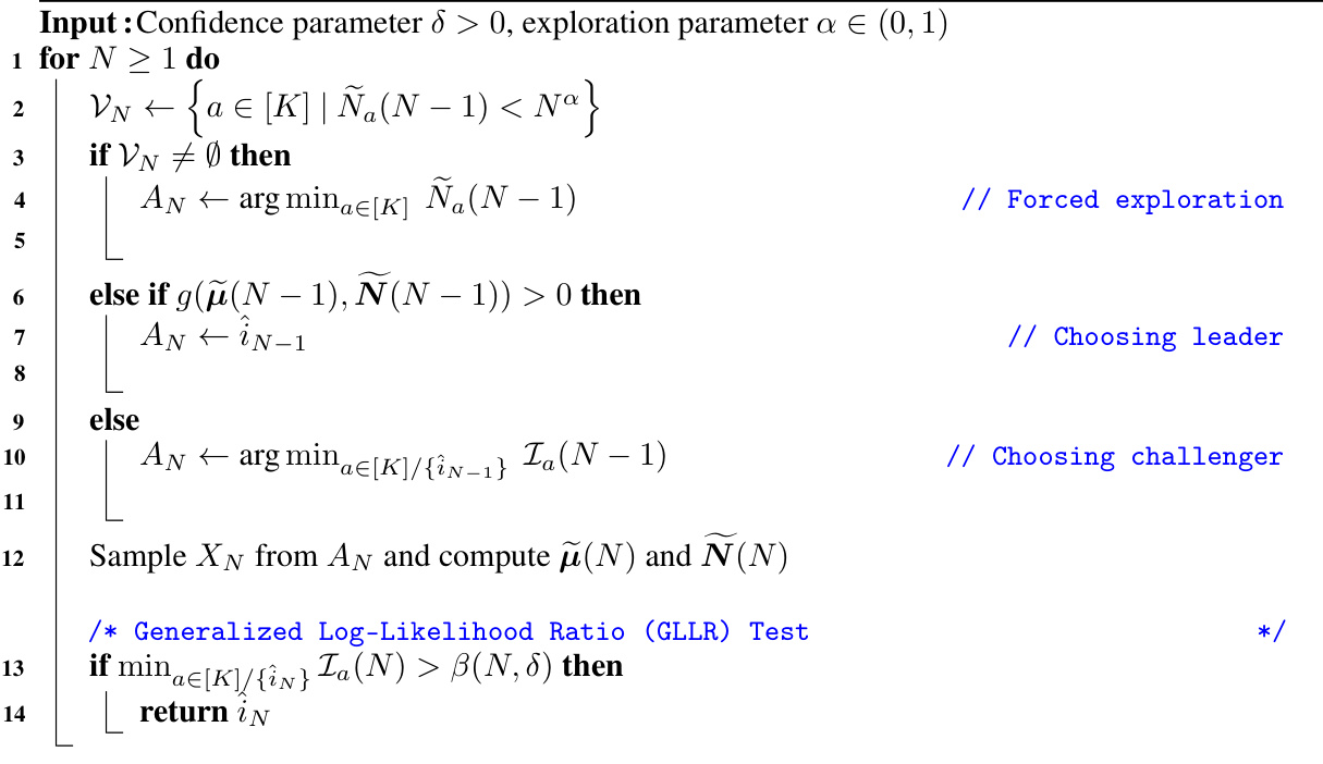
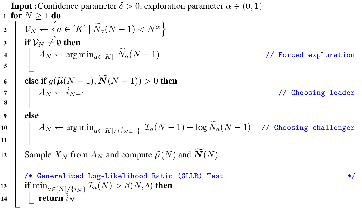
The AT2 (Anchored Top-Two) algorithm presents a novel approach to the best arm identification problem in the multi-armed bandit setting. Its core innovation lies in anchoring the sampling strategy to a threshold function, g, derived from the first-order conditions of the optimal allocation problem. This function dynamically guides the algorithm: if g exceeds the threshold, the empirical best arm is sampled; otherwise, the best challenger arm (identified by a smallest index function) is chosen. This adaptive allocation, unlike traditional top-two methods, is shown to achieve asymptotic optimality by converging to the ideal arm allocation proportions as the number of samples grows. The algorithm’s theoretical properties are rigorously established, drawing upon fluid analysis and the implicit function theorem to characterize its asymptotic behavior. In essence, AT2 offers an improved efficiency and reduced computational cost compared to plug-in methods, by cleverly leveraging the dynamic interplay between the best arm and its challenger through a function-based decision rule.

Asymptotic Optimality

#

The concept of ‘asymptotic optimality’ in the context of best arm identification (BAI) signifies that an algorithm’s performance approaches the theoretical best as a certain parameter (often related to the error probability) tends towards zero. This is a crucial theoretical guarantee, as it assures that the algorithm’s sample complexity (number of samples needed for identification) is essentially as efficient as possible in the limit. The paper likely proves asymptotic optimality by demonstrating that the algorithm’s sample complexity converges to the information-theoretic lower bound as the error probability approaches zero. This involves demonstrating that the algorithm’s allocation of samples across arms closely mirrors the optimal allocation which achieves the theoretical lower bound. Crucially, the use of fluid dynamics and the implicit function theorem likely plays a significant role in this proof. Fluid dynamics simplifies the algorithm’s behavior, providing an approximate continuous evolution rather than a complex discrete sequential process, while the implicit function theorem is likely used to establish the uniqueness and stability of the fluid model’s solution. The achievement of asymptotic optimality does not guarantee excellent finite-sample performance; however, it is a strong theoretical justification that the proposed algorithm is fundamentally well-designed and efficient, particularly when the error probability is extremely low.

IFT Framework

#

The IFT (Implicit Function Theorem) framework, as discussed in the paper, is a crucial mathematical tool used to analyze the asymptotic behavior of the proposed best arm identification algorithms. The paper leverages IFT to establish the existence and uniqueness of a system of ordinary differential equations (ODEs) which describe the limiting fluid dynamics of the algorithms. This fluid model is an idealized representation where the stochasticity of the sampling process is removed, allowing for a more tractable analysis. The IFT’s role is pivotal in proving the convergence of the algorithm’s allocations to the optimal proportions predicted by the theoretical lower bound, as the algorithm’s behavior closely tracks the ODE’s solution. This analysis demonstrates rigor and sophistication, showing that the algorithm’s performance isn’t merely empirical but rooted in strong theoretical foundations. By combining the theoretical lower bounds and fluid approximations, the authors provide a robust justification for the efficacy of their algorithms. The IFT framework is not simply a mathematical tool but a central component in building a rigorous argument for the proposed method’s optimality.

BAI Problem

#

The BAI (Best Arm Identification) problem, central to multi-armed bandit literature, focuses on efficiently identifying the arm with the largest expected reward from a finite set of arms. The challenge lies in balancing exploration (sampling less-certain arms) and exploitation (repeatedly sampling the current best-performing arm). This trade-off is crucial for minimizing the sample complexity while ensuring a high probability of correctly identifying the best arm. Classical approaches often involve computationally intensive methods or rely on asymptotic analyses, limiting practical applicability. The paper explores optimal top-two methods for solving the BAI problem, introducing algorithms that achieve asymptotic optimality while offering enhanced computational efficiency compared to existing techniques. A key contribution is the development of a fluid model to analyze the algorithm’s asymptotic behavior, leveraging the implicit function theorem for rigorous analysis. This novel approach provides a more tractable framework for understanding the complex interplay between exploration and exploitation in the BAI problem, ultimately leading to the design of efficient and optimal algorithms.

More visual insights

#

More on figures

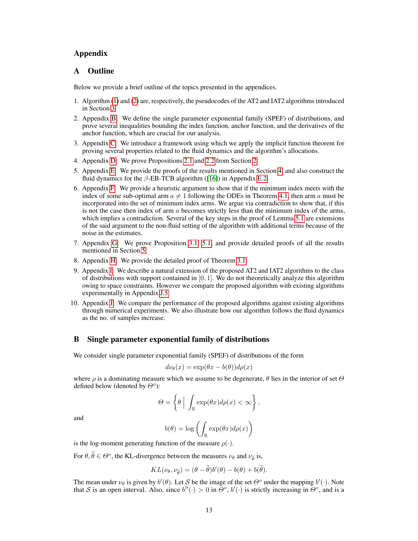
The figure compares the sample complexity of several algorithms for best arm identification. The x-axis represents the beta parameter (probability of pulling the empirical best arm), and the y-axis shows the average sample complexity. The algorithms compared include AT2, IAT2, TCB, ITCB, and variants of the Beta-EB-TCB algorithm. The plot illustrates how the sample complexity varies across different algorithms and beta values.

This figure shows the evolution of the normalized indexes of the sub-optimal arms for the AT2 algorithm, run without the stopping rule, on a single sample path. The normalized indexes are the indexes divided by the total number of samples. The plot shows that once the normalized indexes of the sub-optimal arms get close to each other, they remain close, indicating that the algorithm quickly learns the optimal allocation of samples across the arms. This behavior closely mimics the fluid dynamics described in the paper.

This figure shows the evolution of the normalized indexes of the sub-optimal arms in a 4-armed Gaussian bandit with unit variance and mean vector μ = [10, 8, 7, 6.5]. The plot shows one sample path of the AT2 algorithm without stopping rule. The figure demonstrates that once the normalized indexes are close, they remain close together and the algorithm tracks the fluid path.

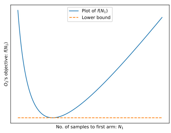
This figure shows an illustrative plot of the objective function f(N1) of the optimization problem O2, as a function of the number of samples allocated to the first arm (N1). The plot shows that f(N1) has a minimum value, representing the optimal allocation of samples. The horizontal dashed line shows the lower bound on the total number of samples required for the problem.

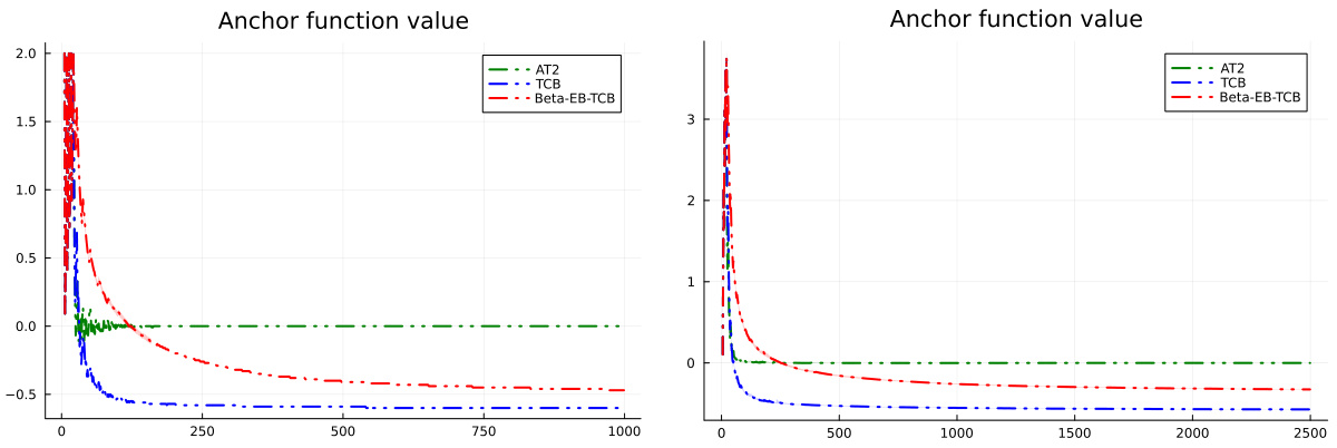
The figure shows the evolution of the anchor function for three different algorithms (AT2, TCB, and Beta-EB-TCB) over 4000 independent sample paths on an easy Gaussian bandit instance. The shaded regions around the solid lines represent the two standard deviations around the mean. The plot illustrates how the anchor function values change over time for the three algorithms, highlighting how AT2 maintains the value close to zero while the other two do not.

This figure compares the sample complexity of different best arm identification algorithms, including AT2, IAT2, TCB, ITCB, and Beta-EB-(I)TCB, across a range of beta values (0.2 to 0.8). The sample complexity represents the average number of samples needed before the algorithm identifies the best arm. The shaded regions around the mean denote two standard deviations.

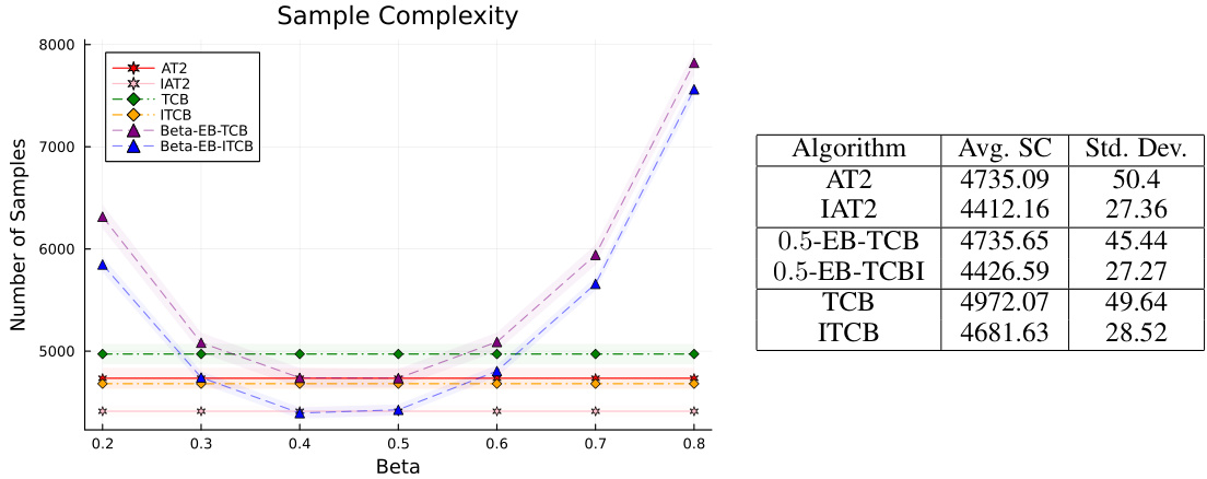
This figure compares the sample complexities of several algorithms for best arm identification, including AT2, IAT2, TCB, ITCB, and Beta-EB-(I)TCB. The x-axis represents the value of beta (β) used in the algorithms, and the y-axis shows the average number of samples required to identify the best arm. The figure shows that the AT2 and IAT2 algorithms generally have lower sample complexity than the other algorithms, particularly for certain values of beta. Error bars are included to show standard deviations.

This figure shows the sample complexity of three algorithms (AT2, TCB, and 0.5-EB-TCB) for different values of delta (error probability) on a Gaussian bandit. It demonstrates how the sample complexity increases as delta decreases, and how AT2 outperforms the other two algorithms, with the difference becoming more pronounced as delta gets smaller.

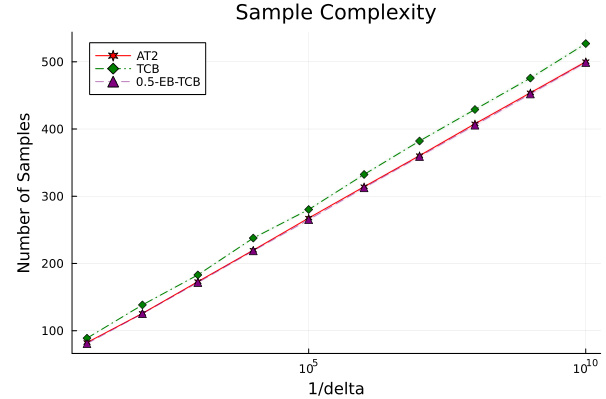
The figure shows the sample complexity of three algorithms (AT2, TCB, and 0.5-EB-TCB) for different values of delta on a Gaussian bandit instance. The sample complexity is the average number of samples needed to identify the best arm with a probability of at least 1-delta. The x-axis represents 1/delta, while the y-axis shows the sample complexity. The plot shows how sample complexity changes as delta decreases (1/delta increases).

This figure shows the sample complexity of three algorithms (AT2, TCB, and 0.5-EB-TCB) as a function of the number of arms (K) in a Gaussian bandit setting. The error probability (δ) is set to 0.001. The y-axis shows the number of samples needed to identify the best arm, and the x-axis shows the number of arms. The plot demonstrates the scalability of the algorithms. All algorithms use the same forced exploration and stopping rules.

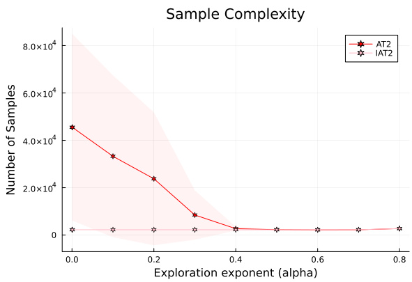
This figure shows the impact of the forced exploration parameter α on the sample complexity of the AT2 and IAT2 algorithms. The x-axis represents the exploration exponent α, and the y-axis shows the number of samples needed to identify the best arm. The results are averaged over multiple independent runs. The plot demonstrates that IAT2’s performance is largely unaffected by α, while AT2’s sample complexity is sensitive to α, particularly in instances where the means of sub-optimal arms are close together. The experiment is conducted on a Gaussian bandit with well-separated means.

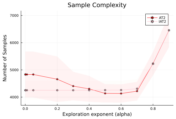
This figure compares the sample complexities of AT2, IAT2, TCB, ITCB, and Beta-EB-(I)TCB algorithms for different beta values on a 4-armed Gaussian bandit with means [10, 8, 7, 6.5] and unit variance. The sample complexity is the average number of samples needed to identify the best arm with probability at least 1-delta. The results are averaged over 4000 independent simulations.

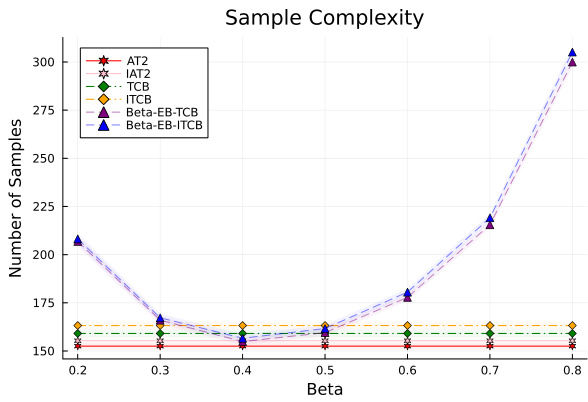
This figure compares the sample complexity of six different algorithms for best arm identification: AT2, IAT2, TCB, ITCB, Beta-EB-TCB, and Beta-EB-ITCB. The x-axis represents the beta value (probability of selecting the empirical best arm), and the y-axis shows the number of samples required to identify the best arm. The figure illustrates how the sample complexity varies across different algorithms and beta values.

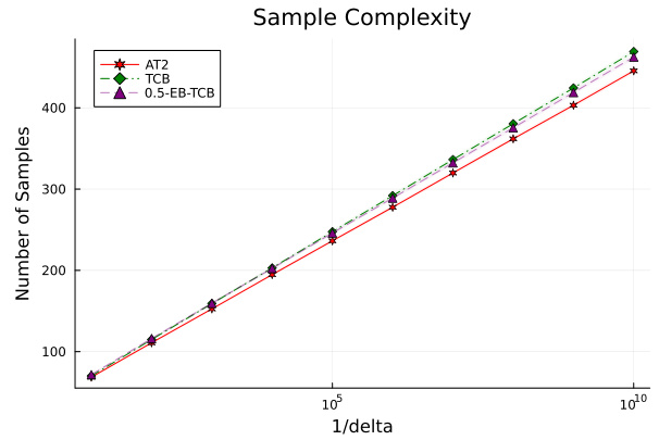
This figure shows the sample complexity of three algorithms, AT2, TCB and 0.5-EB-TCB, as a function of delta (δ). The sample complexity represents the number of samples needed to identify the best arm while guaranteeing that the probability of incorrect selection is below a pre-specified δ. The experiment is conducted on a 4 armed Gaussian bandit with means close to each other, suggesting a harder instance. AT2 consistently shows lower sample complexity across all values of δ, demonstrating its superior performance in this scenario.

Full paper

#