Controlled maximal variability along with reliable performance in recurrent neural networks

↗ OpenReview ↗ NeurIPS Homepage ↗ Chat

TL;DR

#

Key Takeaways

#

Why does it matter?

#

This paper is crucial for researchers exploring neural variability and its role in behavior. It challenges the traditional view that variability hinders performance, introducing a novel principle (NeuroMOP) that maximizes neural variability while maintaining high performance. This opens avenues for building more adaptable and robust artificial systems and for understanding natural systems’ complexity.

Visual Insights

#

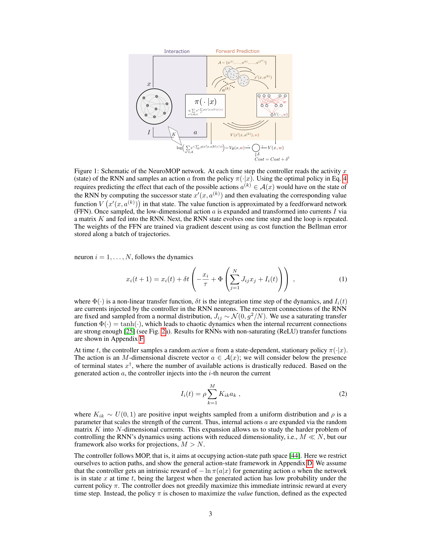
This figure illustrates the architecture of the NeuroMOP network. It shows how a controller (agent) interacts with a recurrent neural network (RNN) environment. The controller samples actions based on the RNN’s current state and uses a feedforward network to approximate a value function that guides its action selection. The goal is to maximize future action-state entropy while avoiding terminal states.

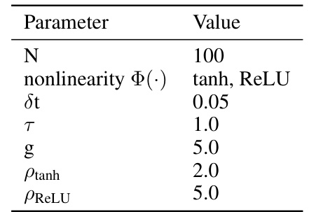
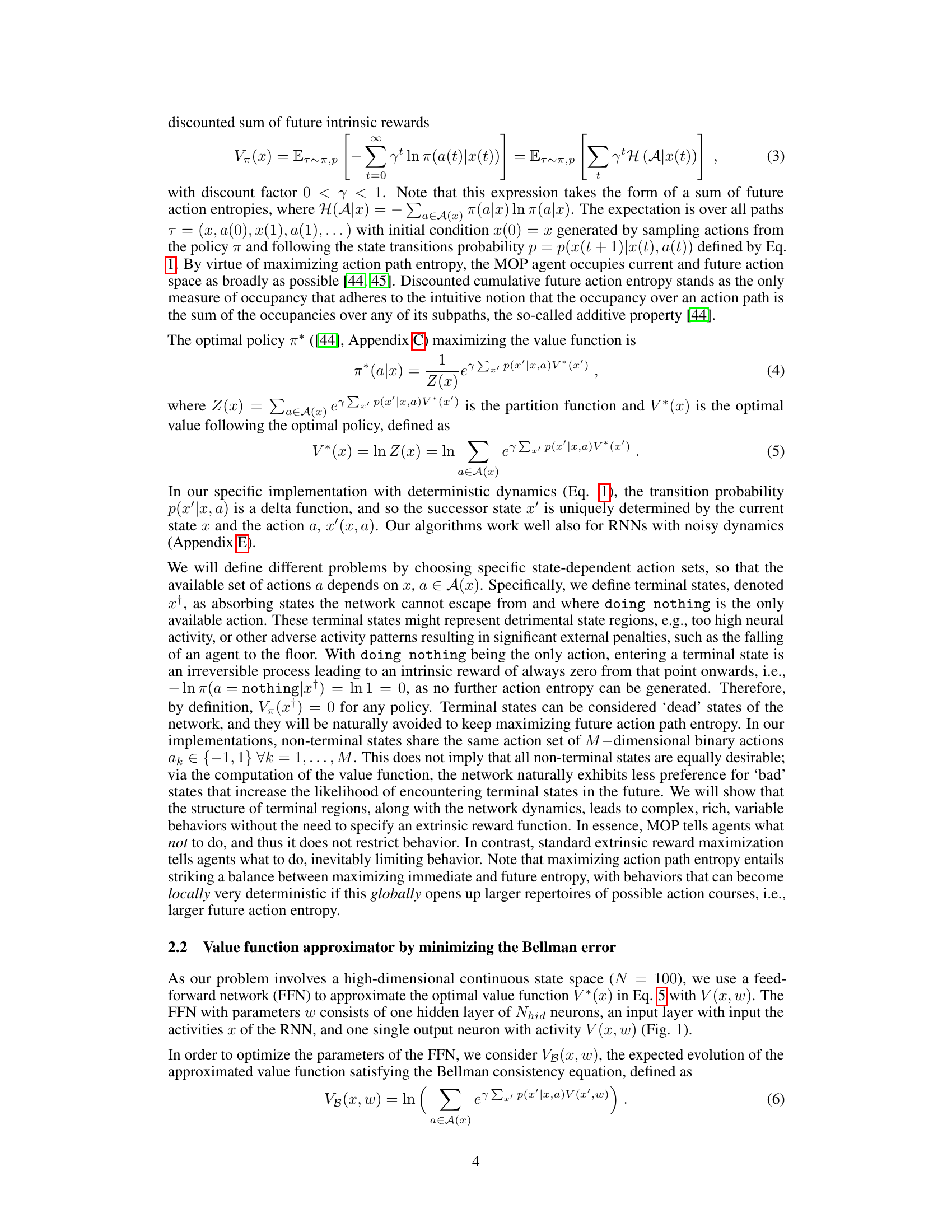
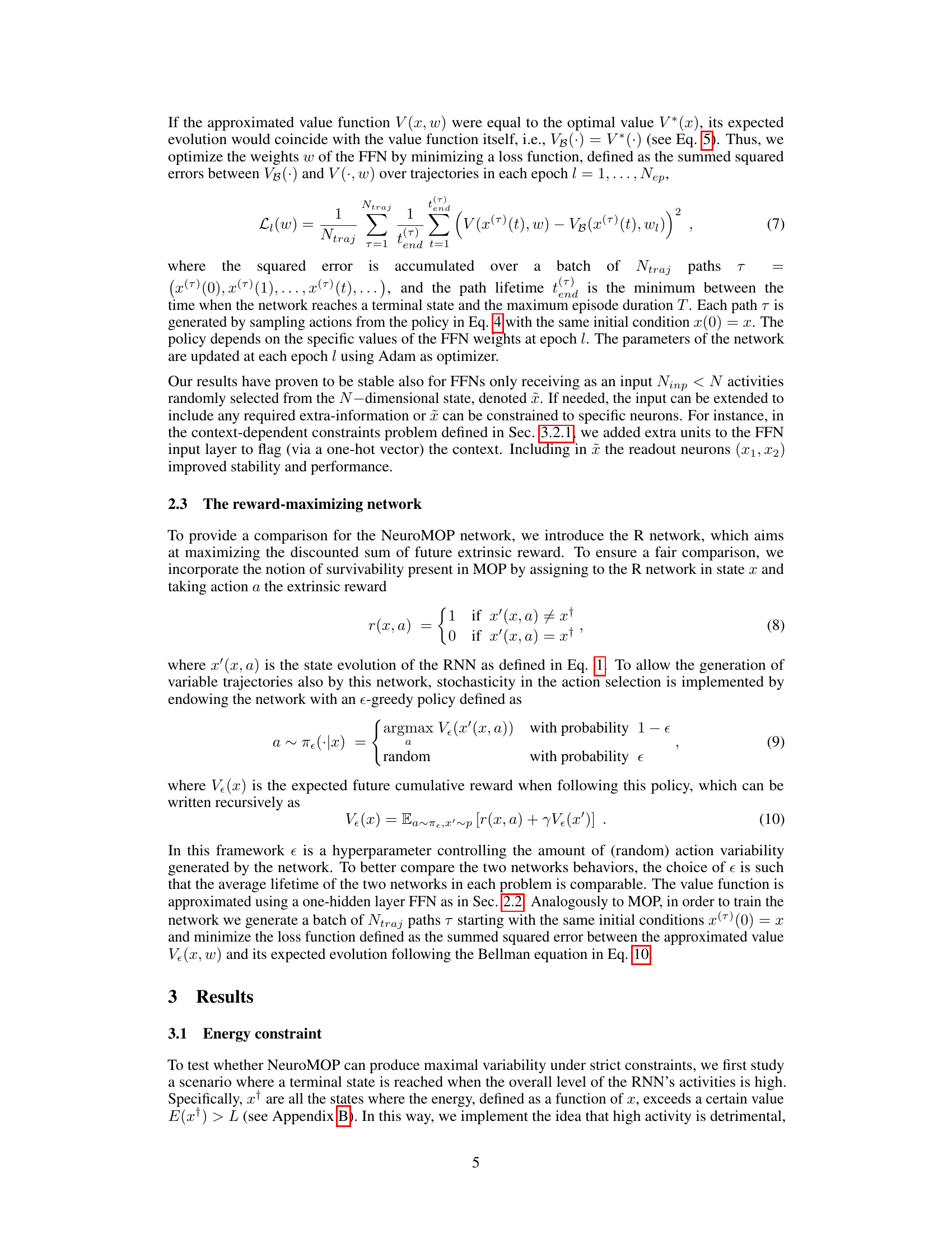
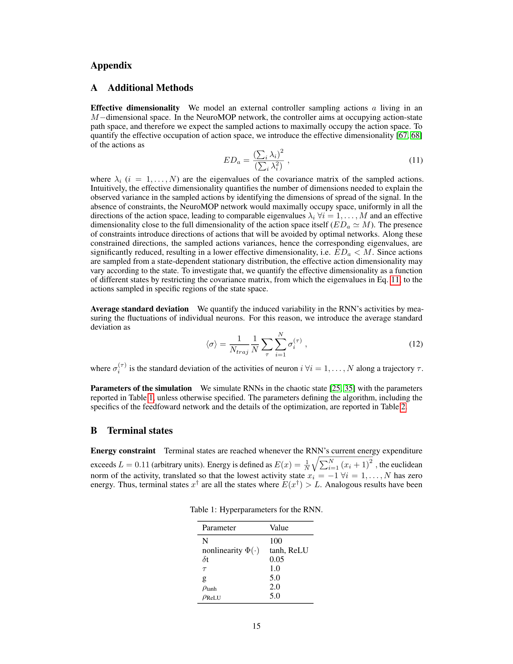
This table lists the hyperparameters used in the recurrent neural network (RNN) simulations. The parameters include the number of neurons (N), the type of nonlinear activation function (tanh or ReLU), the integration time step (dt), the time constant (τ), the scaling of recurrent connections (g), and parameters specific to tanh and ReLU activation functions (ρ_tanh and ρ_ReLU). These parameters control various aspects of the RNN’s dynamics, such as the level of chaos and the network’s overall behavior.

In-depth insights

#

NeuroVariability

#

NeuroVariability, a concept central to the provided research, explores the multifaceted nature of variability in neural activity and its implications for behavior. The study challenges the traditional view that neural variability is detrimental to performance, suggesting instead that controlled maximal variability is key to flexible and adaptive behavior. This perspective is supported by the introduction of the NeuroMOP principle, which frames neural variability as a means to maximize future action-state entropy. This concept emphasizes the intrinsic motivation of the nervous system to explore its entire dynamic range, generating diverse activity patterns while avoiding terminal states. The work uses recurrent neural networks to illustrate how a controller can inject currents to maximize entropy and solve complex tasks while maintaining high variability. NeuroMOP offers a novel framework for understanding neural variability, reconciling stochastic and deterministic behaviors, highlighting how the system dynamically switches between these modes to adapt to constraints. The research thereby provides a compelling theoretical and computational model of how neural variability is not mere noise, but a fundamental mechanism contributing to robust and flexible behavior.

NeuroMOP Agent

#

A NeuroMOP agent is a novel computational entity designed to maximize future action-state entropy in a neural network. It operates by injecting currents (actions) into a recurrent neural network (RNN) with fixed random weights, effectively acting as a controller to shape the network’s dynamic activity. Unlike traditional reinforcement learning agents focused on maximizing rewards, the NeuroMOP agent’s intrinsic motivation is to generate maximal neural variability while adhering to constraints, such as avoiding terminal states. This principle, maximizing occupancy in the action-state space, leads to a unique approach to learning where exploration is prioritized over exploitation. The agent’s flexibility to switch between stochastic and deterministic modes is key to achieving high performance and variability simultaneously. This makes it a unique model for understanding neural variability and its role in flexible behavior.

Maximal Entropy

#

The concept of “Maximal Entropy” in the context of neural networks, especially recurrent ones, is a fascinating exploration of how to maximize neural variability while maintaining high network performance. It challenges the conventional approach of suppressing variability to improve performance, instead proposing that maximal variability, carefully structured to avoid negative outcomes, is beneficial. The principle seems to promote exploration of the network’s entire dynamical range, enabling the generation of diverse behavioral repertoires. This is achieved by a controller aiming to maximize future action-state entropy, essentially encouraging the system to explore all possible activity patterns without ending up in detrimental states. This approach contrasts with traditional reinforcement learning methods which often aim for deterministic policies after learning. The introduction of terminal states, defining undesirable activity patterns, is crucial in guiding the network towards beneficial variability and preventing catastrophic failures. The exploration of this ‘Maximal Entropy’ principle seems promising in creating more robust and flexible neural networks, and its biological relevance is noteworthy. Further research into understanding how this principle applies to real biological systems could be particularly insightful.

RNN Dynamics

#

Recurrent Neural Networks (RNNs) are known for their ability to model sequential data by maintaining an internal state that is updated at each time step. The dynamics of an RNN are determined by the interactions between its units, and the type of activation function used. Understanding RNN dynamics is crucial for interpreting their behavior and designing effective architectures. The paper likely explores various aspects of RNN behavior, such as the impact of different activation functions on the stability and capacity of the network, exploring chaotic behavior, investigating the role of noise and stochasticity, and how different training methods can lead to different dynamical regimes. An important aspect might be the role of external inputs and how they interact with the internal state to shape network dynamics. This could encompass the interaction with controllers which use an optimal policy to manipulate the RNN state. The study could involve analyzing the effect of energy constraints on the overall dynamics, with attention to how the network balances maximal variability and reliable performance under such limitations. The concept of terminal states, defined as absorbing states where no further entropy can be generated, is crucial in navigating the RNN’s state space. Such insights can lead to novel theoretical and practical frameworks for RNNs.

Future Research

#

Future research directions stemming from this work on NeuroMOP could explore several key areas. Extending the framework to incorporate policy learning using methods like actor-critic algorithms would enhance the model’s practicality. Investigating the impact of different noise models and transfer functions on network behavior, particularly in relation to variability, is crucial. The effects of various energy constraints and their biological plausibility deserve further examination, connecting the theoretical model to real-world neural limitations. Finally, applying NeuroMOP to more complex tasks and environments would validate its effectiveness and generalizability across different neural architectures, potentially revealing deeper insights into the functional role of neural variability in biological systems. The framework could also be tested for robustness across various RNN parameters and its adaptation to diverse behavioral paradigms.

More visual insights

#

More on figures

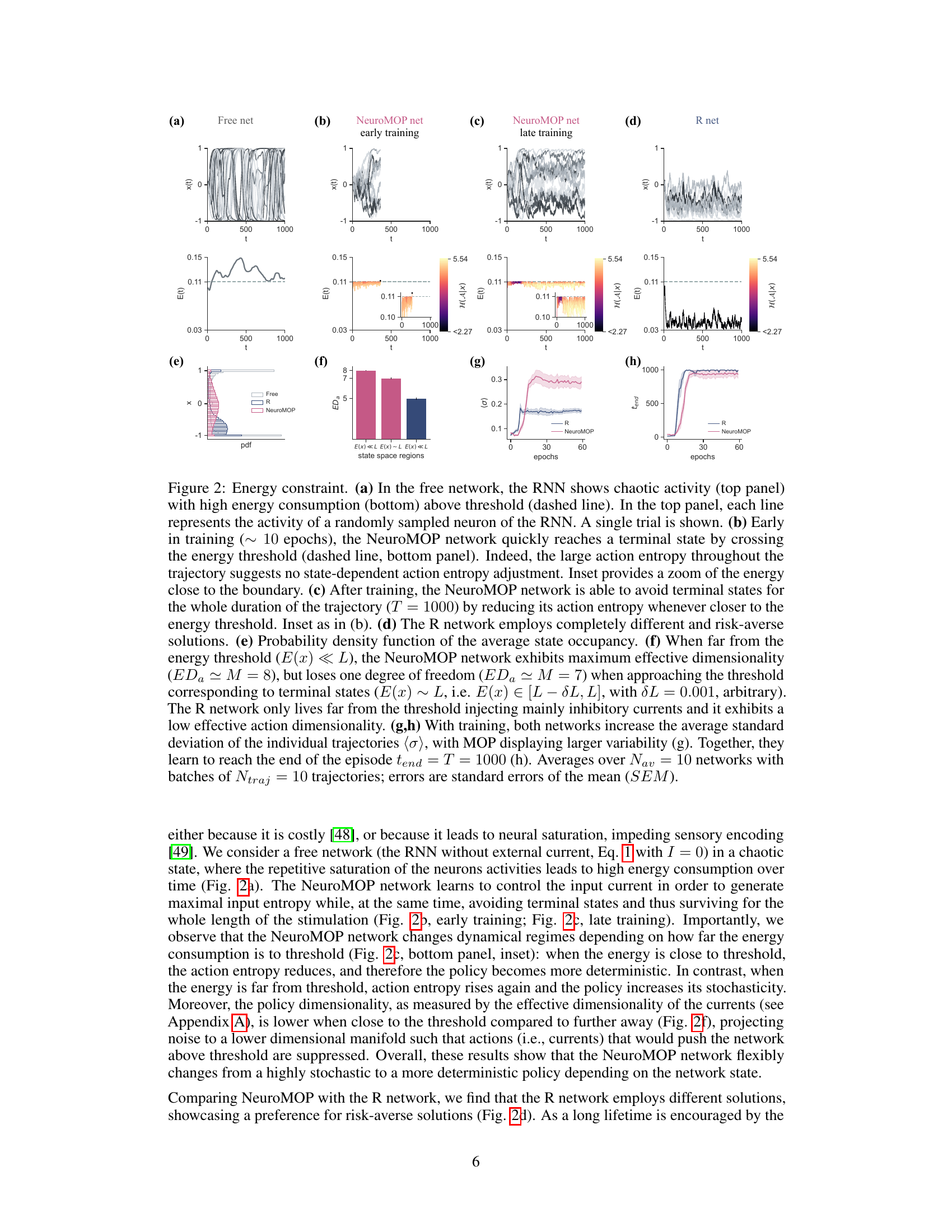
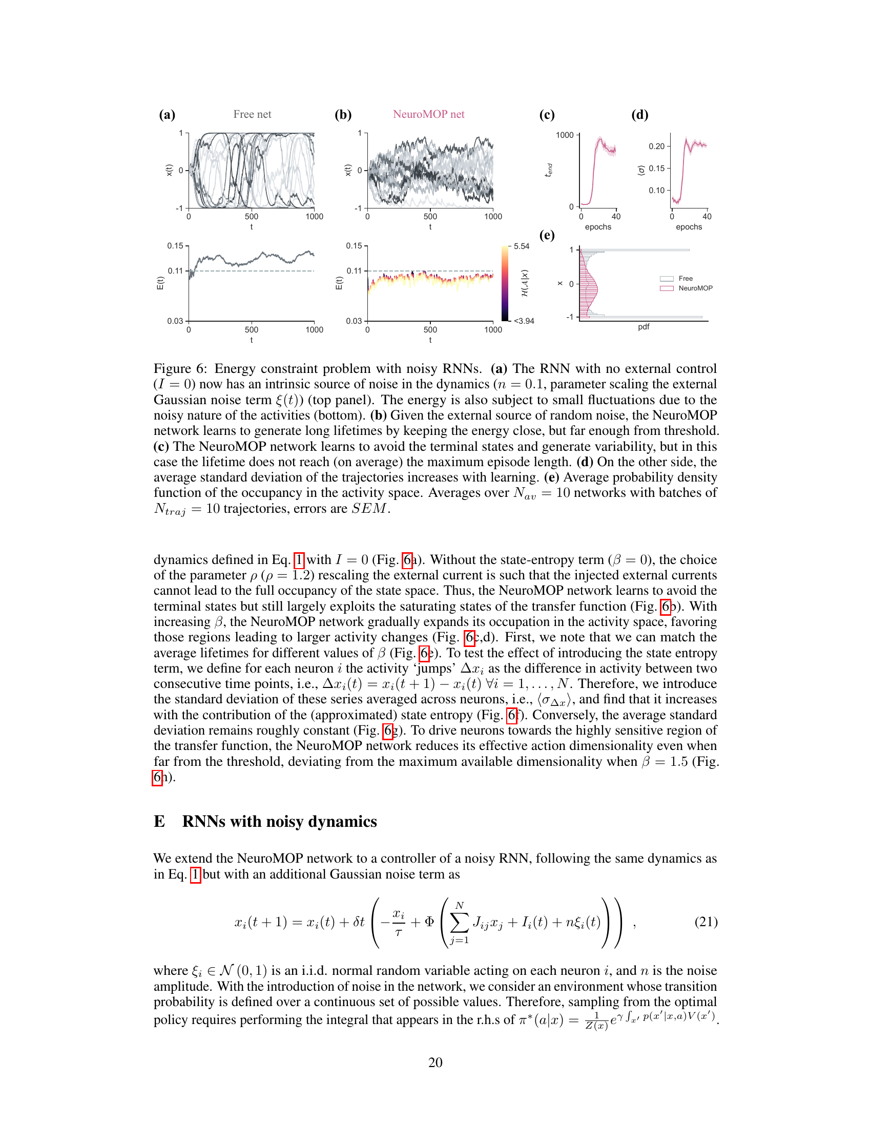
This figure compares the performance of three different network approaches under energy constraints. The free network exhibits chaotic activity and high energy consumption. The NeuroMOP network learns to avoid terminal states and maintains high variability, adapting its action entropy based on proximity to the threshold. The R network employs a risk-averse strategy, maintaining low variability and low energy consumption. The figure shows neural activities, energy levels, action entropy, probability distributions, effective dimensionality, and variability metrics, illustrating how the different networks achieve their objectives.

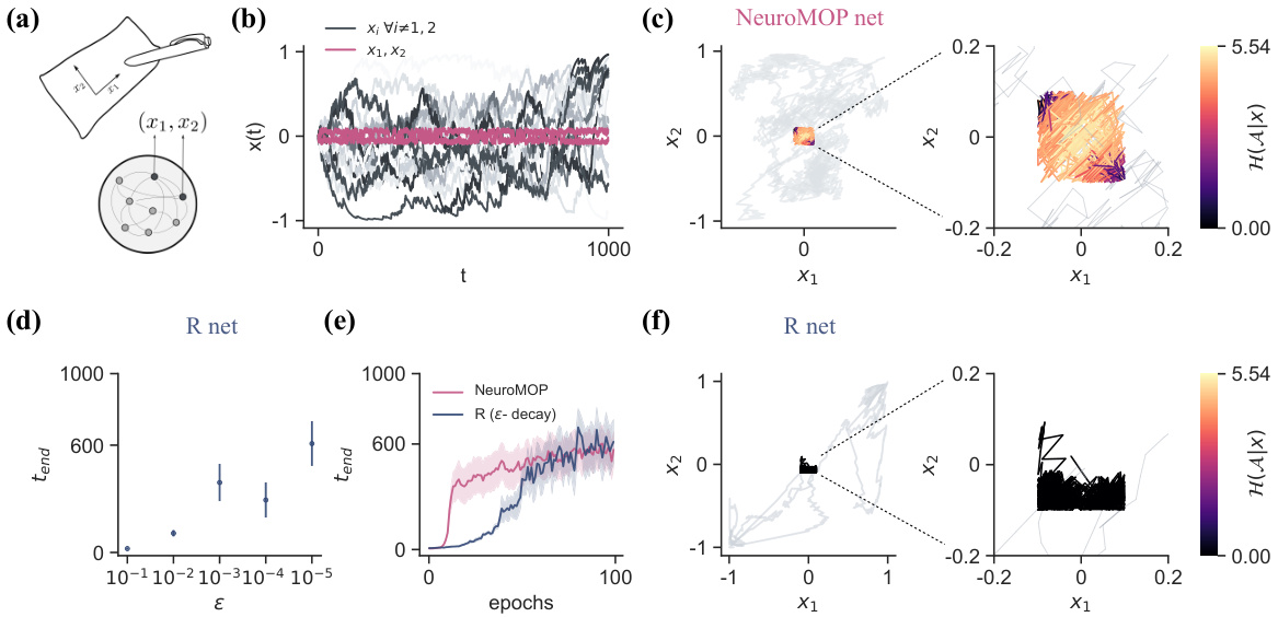
This figure compares the NeuroMOP and R networks in a task where terminal states are defined as the boundaries of a square in the activity space of two selected neurons. NeuroMOP successfully confines the activities within the square while exploring the interior. The R network, using an epsilon-greedy policy, fails to do so unless epsilon is extremely low. The figure shows trajectories, action entropy, and effective dimensionality for both methods.

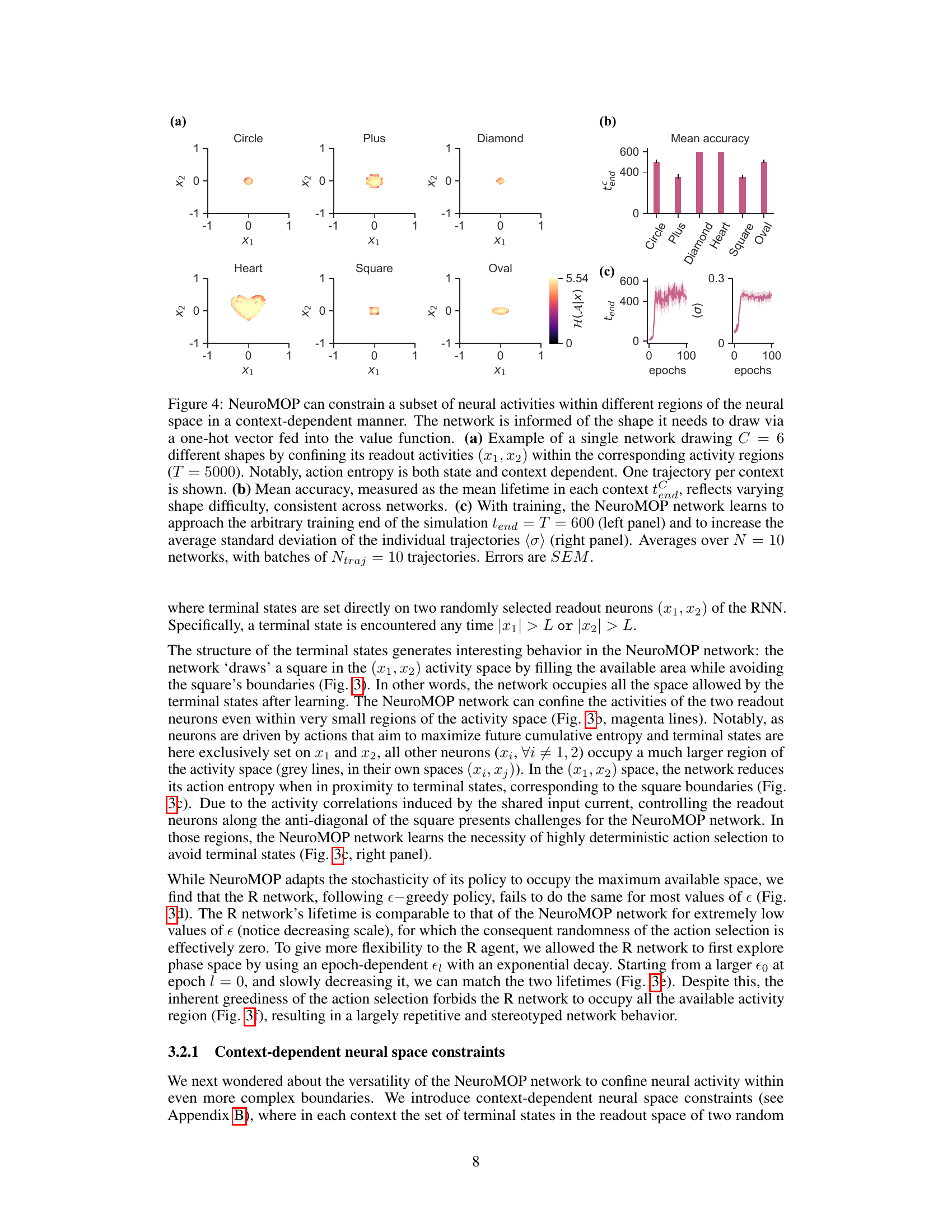
This figure demonstrates the NeuroMOP network’s ability to constrain neural activities within different regions of the neural space in a context-dependent manner. The network receives a one-hot vector indicating the shape it should draw. Subplots show examples of the network drawing six different shapes by confining its readout activities within the corresponding activity regions. The figure also quantifies the mean lifetime (accuracy) across the different shapes and shows the increase in average standard deviation of the trajectories with training, highlighting the network’s ability to achieve maximal variability while performing a task.

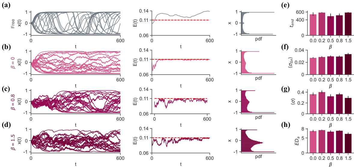
This figure shows the results of experiments conducted to test the effect of introducing a state-entropy reward term to the NeuroMOP network. The experiments vary the β parameter, which regulates the amount of state entropy in the reward function. The results demonstrate how different β values affect network behavior, including occupancy of saturating versus non-saturating neural activity states, average lifetime, variability of neural activity, and effective dimensionality of the action signals. These results highlight the impact of state-entropy on the control of neural activity and the flexibility of the NeuroMOP approach.

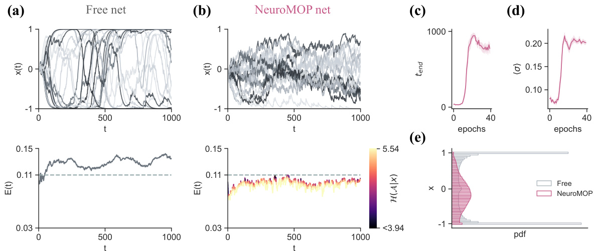
This figure compares the performance of the NeuroMOP network and a reward-maximizing (R) network in an energy constraint scenario. The NeuroMOP network effectively avoids terminal states by adaptively adjusting its action entropy, while the R network employs risk-averse strategies. The NeuroMOP network shows greater variability and higher effective dimensionality.

This figure compares the performance of the NeuroMOP network and a reward-maximizing (R) network in a scenario with an energy constraint. The NeuroMOP network learns to avoid terminal states while maintaining high activity variability, adaptively adjusting its action entropy based on proximity to the energy threshold. The R network adopts a more risk-averse strategy.

This figure shows the results of applying the NeuroMOP algorithm to the classic cartpole balancing problem. Panel (a) depicts a schematic of the cartpole system. Panel (b) displays a heatmap showing the probability density of the cart’s position and pole angle over time. The MOP network successfully balances the pole while maintaining variability in its state. Panel (c) illustrates how the network’s performance (measured as the length of time it successfully balances the pole) improves as the value function is trained.

This figure demonstrates the NeuroMOP network’s ability to navigate a complex environment consisting of two open areas connected by a narrow passage. The network successfully traverses the corridor while maintaining low action entropy, highlighting its adaptability. The color coding in (a) represents the action entropy across the trajectory. The (b) graph shows how the average lifetime of the network improves over epochs.

This figure shows how adding an extrinsic reward to the NeuroMOP model affects its behavior in a constrained neural space. The model’s activity is confined to a square, and an additional reward is given for activity within a smaller inner square. Two different reward weights (μ) are shown: (a) μ = 0.1, where the reward has a minor influence, and (b) μ = 0.5, where the reward strongly influences the activity, causing it to be concentrated in the smaller rewarded area. The plots show the probability density of activity within the space and the lifetime (how long the model avoids terminal states) over training epochs.

More on tables

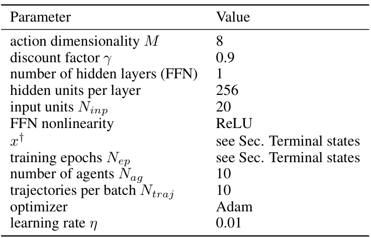
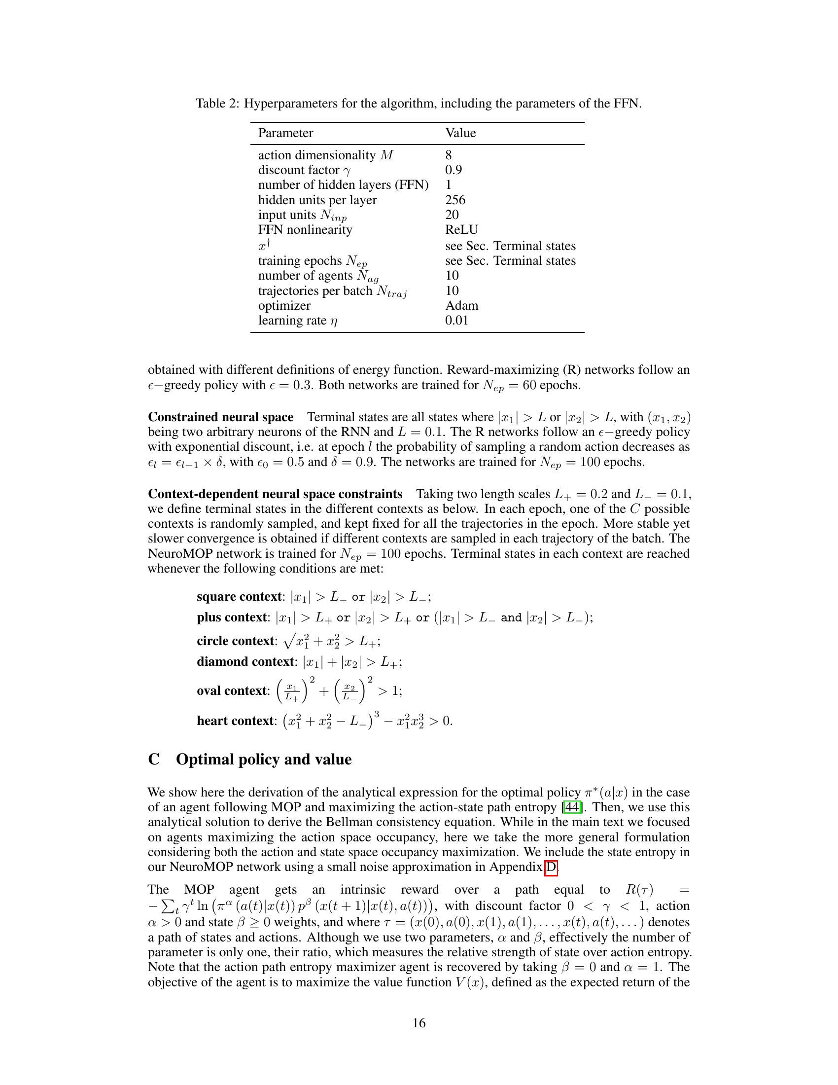
This table lists the hyperparameters used in the NeuroMOP algorithm and its associated feedforward neural network (FFN). It specifies values for parameters controlling the dimensionality of the actions, the discount factor, FFN architecture (number of layers and hidden units), the input units to the FFN, the activation function of the FFN, the definition of terminal states, training parameters (epochs, number of agents, trajectories per batch, and optimizer), and the learning rate. The values reflect the settings used in the experiments detailed in the paper.

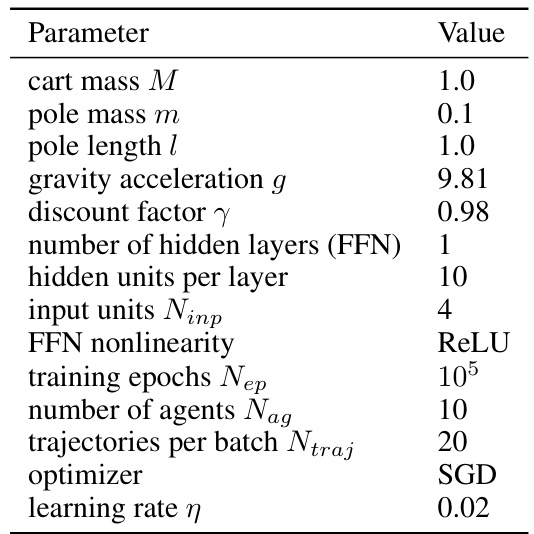
This table lists the hyperparameters used in the cartpole balancing experiment. These parameters define the physical properties of the cartpole (mass, length, gravity), the algorithm’s settings (discount factor, number of hidden layers in the feedforward network approximating the value function), and the training process (number of training epochs, number of agents used for training, number of trajectories per batch, optimizer used (SGD), and the learning rate).

Full paper

#