↗ OpenReview ↗ NeurIPS Homepage ↗ Chat
TL;DR#
Dimensionality reduction (DR) for visualization is crucial for exploratory data analysis but faces challenges with existing methods such as t-SNE (distortions) and PCA (global collapse). Hierarchical DR offers a multiscale view but existing methods are either computationally expensive or lack interpretability.
This paper introduces PCA tree, a novel hierarchical DR model that uses a sparse oblique tree for projection and local PCAs in leaves. Joint optimization of parameters ensures monotonic error decrease, enabling scalability. Experiments show PCA trees effectively identify low-dimensional structures and clusters, showcasing superior interpretability and efficiency compared to t-SNE and UMAP.
Key Takeaways#
Why does it matter?#
This paper is crucial for researchers in dimensionality reduction and data visualization. It introduces a novel, interpretable, and scalable method (PCA tree) that overcomes limitations of existing techniques. The hierarchical approach provides valuable insights, and the algorithm’s efficiency opens avenues for large-scale data analysis. Its interpretability enhances the model’s trustworthiness.
Visual Insights#

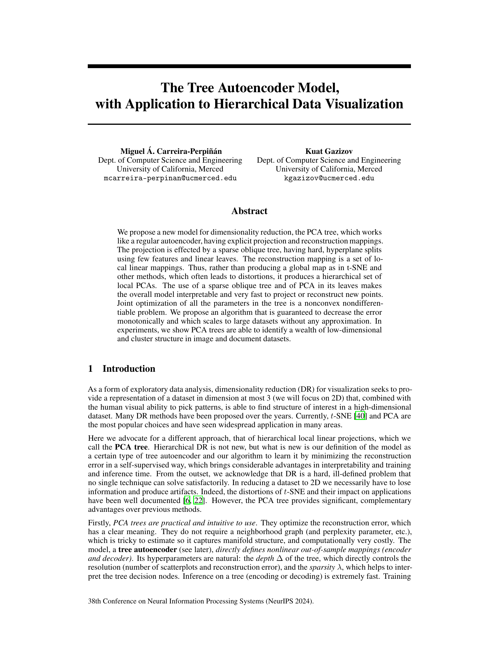
This figure illustrates the PCA tree autoencoder model. The left panel shows a simplified representation of the model as a tree with an encoder (projection) and decoder (reconstruction) at each node. The input data x is processed by the encoder, which uses a tree structure to route x to one of the leaves. Each leaf has its own PCA, projecting the data into a lower-dimensional space (2D in this example). The resulting latent vector (z) is then passed to the decoder, which reconstructs the output y. The right panel provides a 3D visualization of the data space being partitioned by the tree into four 2D spaces (one for each leaf), each with its own local PCA.

This table provides a summary of the characteristics of the five datasets used in the paper’s experiments. It shows the number of samples (N), the dimensionality of the data (D), and the number of classes (K) for each dataset: MNIST, Fashion MNIST, Letter Recognition, 20 Newsgroups, and Amazon Reviews.
In-depth insights#
PCA Tree Model#
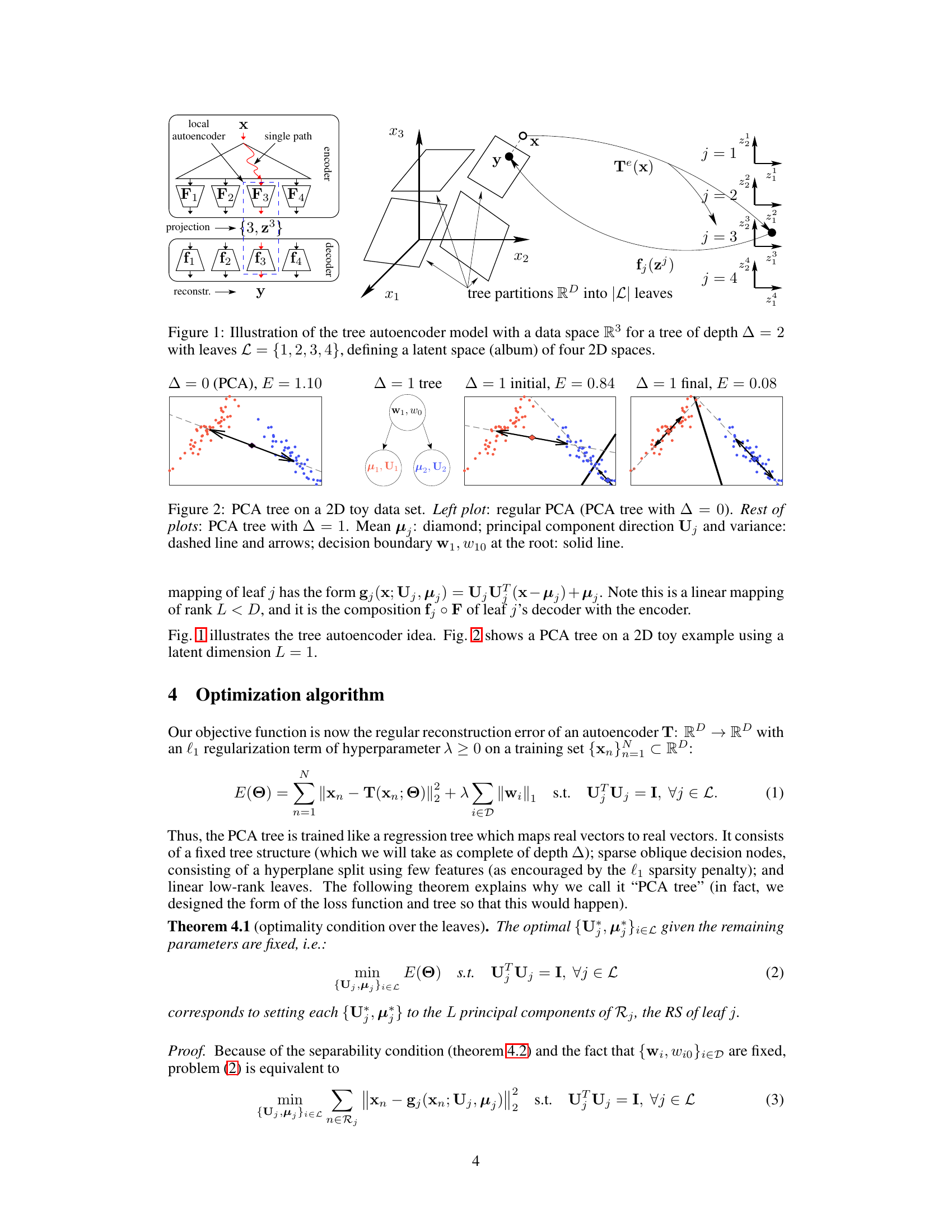
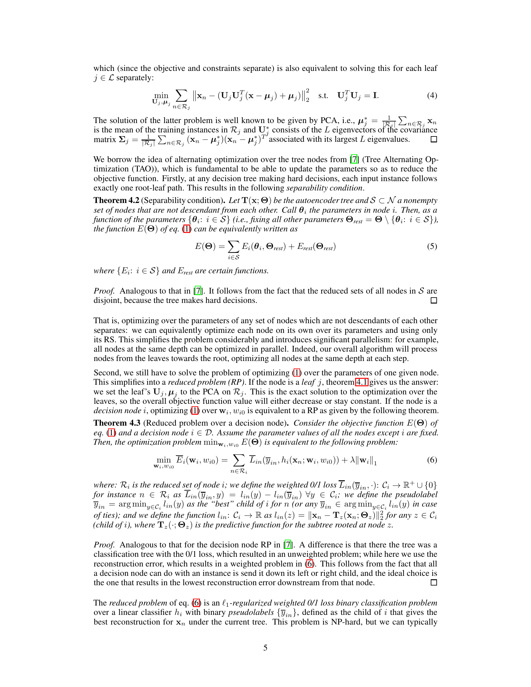
The PCA Tree model presents a novel approach to dimensionality reduction, combining the strengths of hierarchical tree structures and local Principal Component Analyses (PCAs). Instead of a global projection like traditional PCA or t-SNE, it employs a tree to partition the data space into smaller regions. Each leaf node then performs a PCA, resulting in a set of local, low-dimensional representations. This hierarchical structure offers significant advantages, including improved interpretability due to the explicit partitioning and the ease of visualizing local data clusters. Computational efficiency is another key benefit, as the tree structure allows for fast encoding and decoding of new data points. The model’s nonconvex optimization is addressed via a proposed algorithm that monotonically decreases the reconstruction error, ensuring stable training and scalability to large datasets. The approach presents a compelling alternative to traditional methods for dimensionality reduction, particularly in scenarios where interpretability and efficiency are paramount.
Hierarchical DR#
Hierarchical dimensionality reduction (DR) methods offer a multiscale approach to data visualization, addressing limitations of single-scale methods like PCA and t-SNE. Soft hierarchical DR techniques employ probabilistic models, such as soft trees, to allow an instance to traverse multiple paths in the hierarchy, creating a blended representation that is often differentiable but can sacrifice interpretability. Hard hierarchical DR methods utilize tree structures, where each instance follows a single path. This approach, often faster and more interpretable, partitions the data into nested subsets, which can reveal multi-level structure. A key challenge lies in optimizing the tree structure and local linear projections simultaneously to minimize reconstruction error, which often involves non-convex, non-differentiable objective functions. The choice between soft and hard approaches hinges on the tradeoff between differentiability/optimization ease and interpretability/efficiency.
Interpretable Maps#
Interpretable maps in the context of dimensionality reduction aim to visualize high-dimensional data in a way that is both accurate and easily understood. Unlike traditional methods that might produce visually appealing but complex projections, interpretable maps prioritize clarity and insight. This involves techniques that reveal meaningful structure, such as clear cluster separation, relationships between data points, and potentially the identification of important features driving the visualization. Effective interpretability often leverages inherent characteristics of the data or employs techniques that allow for easy inference of the underlying data structure. For instance, visualizations might use color-coding to represent categories, label clusters with meaningful descriptions, or display feature weights to illustrate their importance in the mapping. The goal is to facilitate human understanding and enable discovery of patterns that might otherwise be hidden in a complex dataset, making it a crucial aspect of exploratory data analysis and supporting the development of trust in AI models.
Scalable Training#
Scalable training in machine learning models is crucial for handling massive datasets. The paper likely details optimization strategies that allow the model to train efficiently even with a large number of data points and dimensions. Parallel processing techniques, where computations are distributed across multiple processors, are frequently employed for improved speed and scalability. Efficient algorithms that reduce computational complexity, perhaps through approximations or clever data structures like tree-based methods, are also key for handling big data. The authors might demonstrate the linear or sublinear scaling of the training time with respect to dataset size, indicating successful scalability. A critical aspect is parallelizability, ensuring that different parts of the training process can be performed concurrently. The discussion likely includes a comparison with existing DR methods, highlighting the relative advantages in training efficiency and scalability offered by the proposed approach. Finally, interpretability is a valuable characteristic; thus, the paper might emphasize how the scalable training procedure doesn’t compromise model interpretability.
Future Research#
Future research directions stemming from this PCA tree model could explore several promising avenues. Extending the tree structure to handle more complex non-linear relationships in higher dimensional data is crucial. Investigating alternative tree structures beyond the oblique trees used here, such as those incorporating more sophisticated splitting criteria or allowing for more flexible leaf models, could improve performance and interpretability. Developing more efficient optimization algorithms that scale to truly massive datasets is also essential, potentially by leveraging distributed computing or advanced approximation techniques. In addition to its use in visualization, the model’s potential for applications in other areas, such as dimensionality reduction for machine learning tasks, needs to be thoroughly explored, examining its performance in settings where interpretability is paramount. Finally, a more comprehensive comparison with other state-of-the-art dimensionality reduction techniques should be performed, focusing on a wider range of datasets and metrics to rigorously establish the model’s strengths and weaknesses.
More visual insights#
More on figures

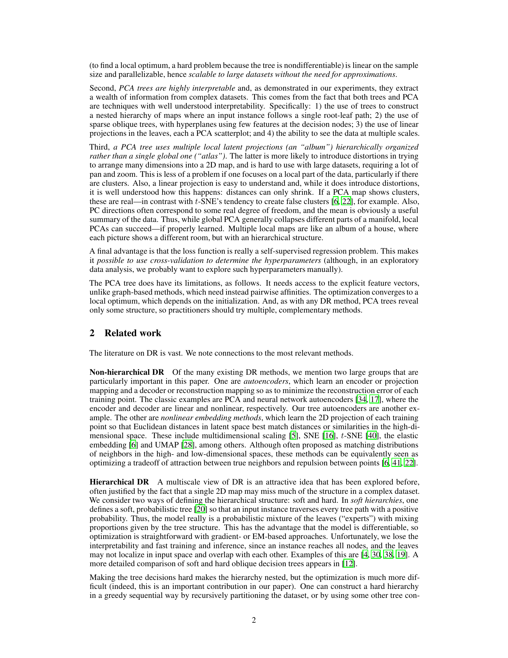
This figure shows a comparison of PCA and PCA tree on a 2D toy dataset. The leftmost plot shows the result of applying regular PCA (which is equivalent to a PCA tree with depth ∆=0). The other three plots show the results of applying a PCA tree with depth ∆=1. Different stages of the training are shown (initial and final). For the PCA tree, the mean (μj), principal component direction (Uj), and variance of each leaf are shown, along with the decision boundary (w₁, w10) at the root node. The figure illustrates how the PCA tree partitions the data space and fits local PCA models to each partition.

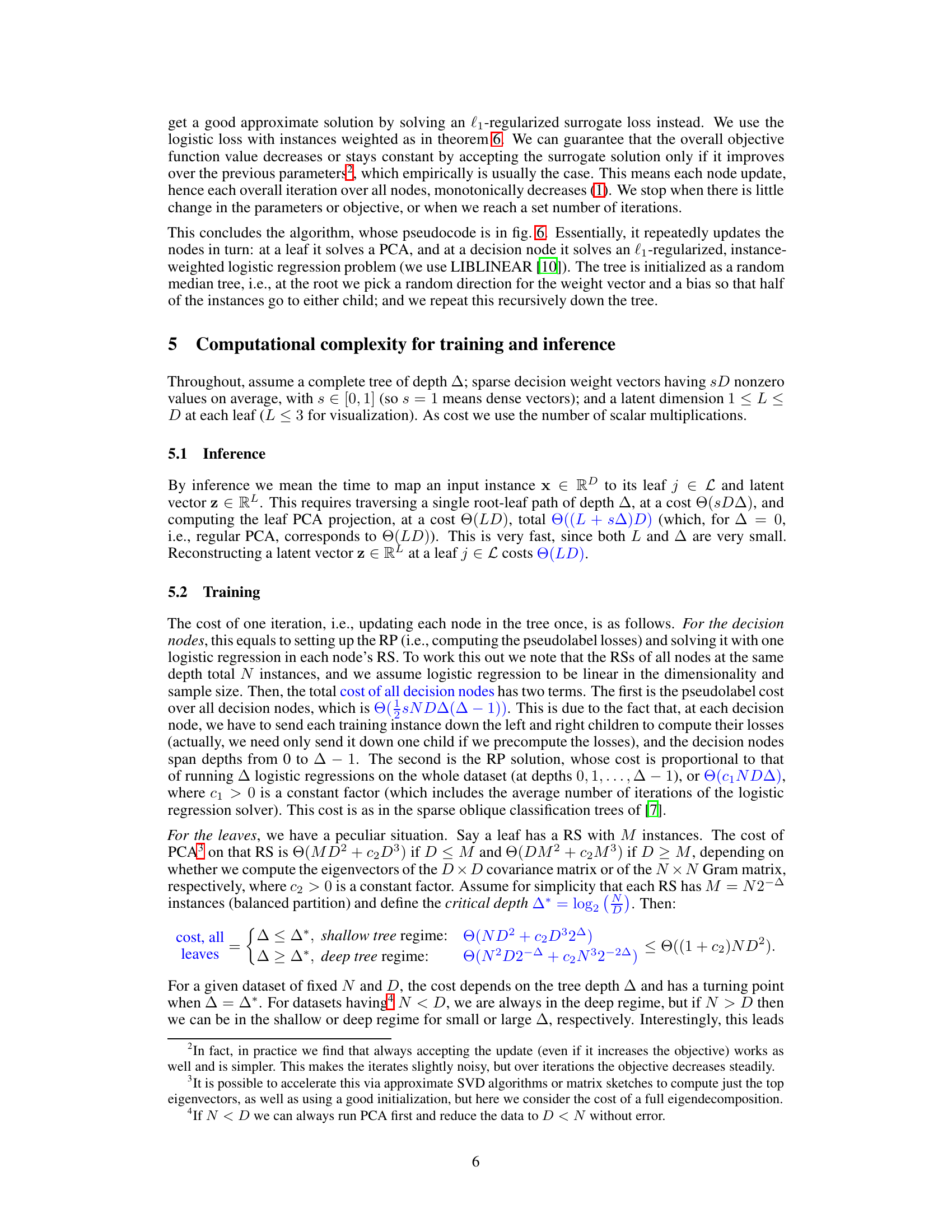
This figure presents a comprehensive evaluation of the PCA tree algorithm’s performance and scalability. The first two plots illustrate the training time per iteration for the MNIST dataset at varying depths (∆) and dimensions (D), comparing theoretical and actual results. The third plot compares the training time of PCA trees against t-SNE and UMAP for different sample sizes (N), highlighting PCA tree’s superior scalability. The final two plots showcase the convergence of the objective function over iterations across different datasets and depths.

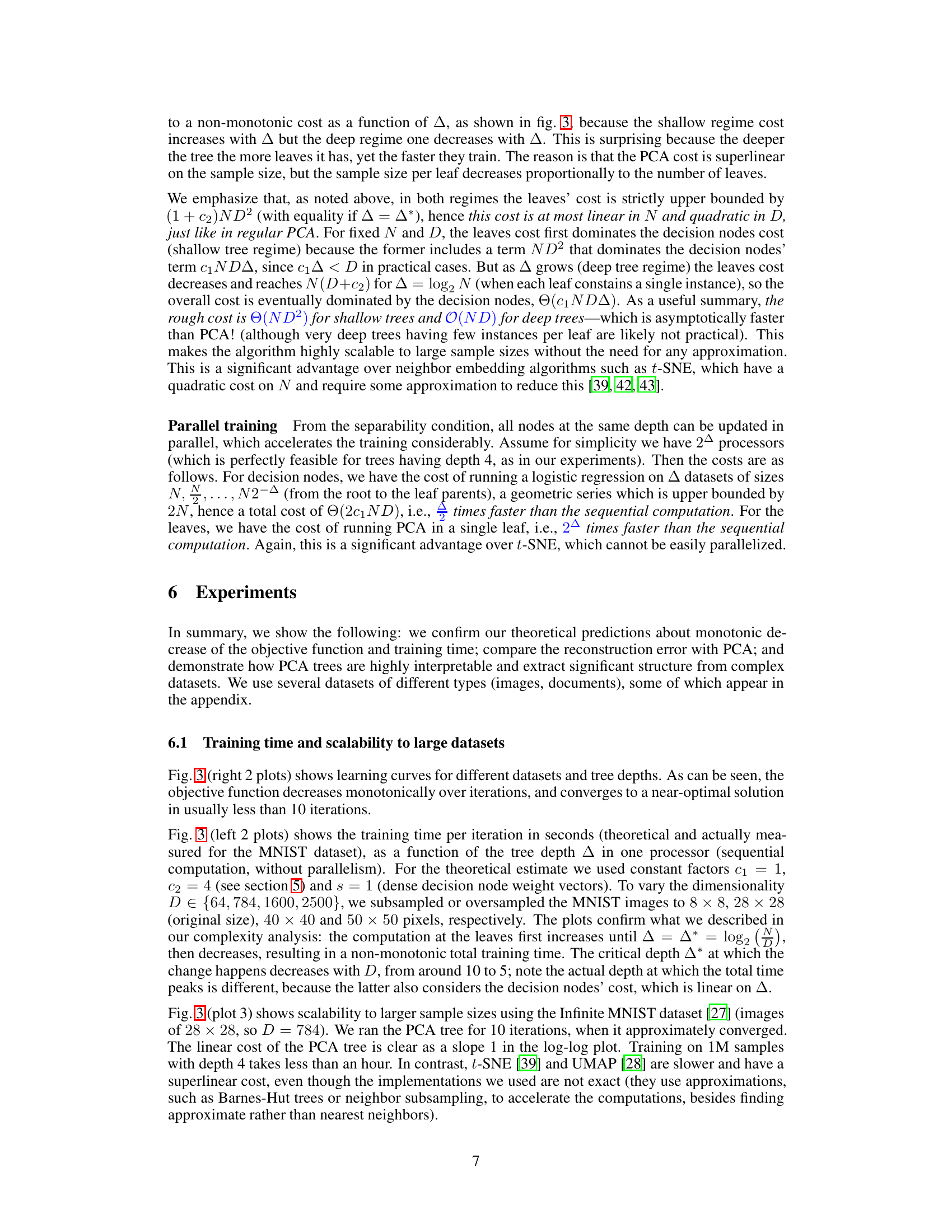
This figure compares the reconstruction error of PCA and PCA tree for Fashion MNIST and 20newsgroups datasets. The x-axis represents the number of principal components (L) used in PCA, and the y-axis shows the squared reconstruction error per sample. For the PCA tree, the number of principal components is fixed at L=2 in each leaf, and the depth of the tree (Δ) is varied. The plots illustrate that the PCA tree achieves a lower reconstruction error than PCA, especially when the number of principal components in PCA is relatively small. The different lines for the PCA tree show how the reconstruction error changes with varying tree depths.

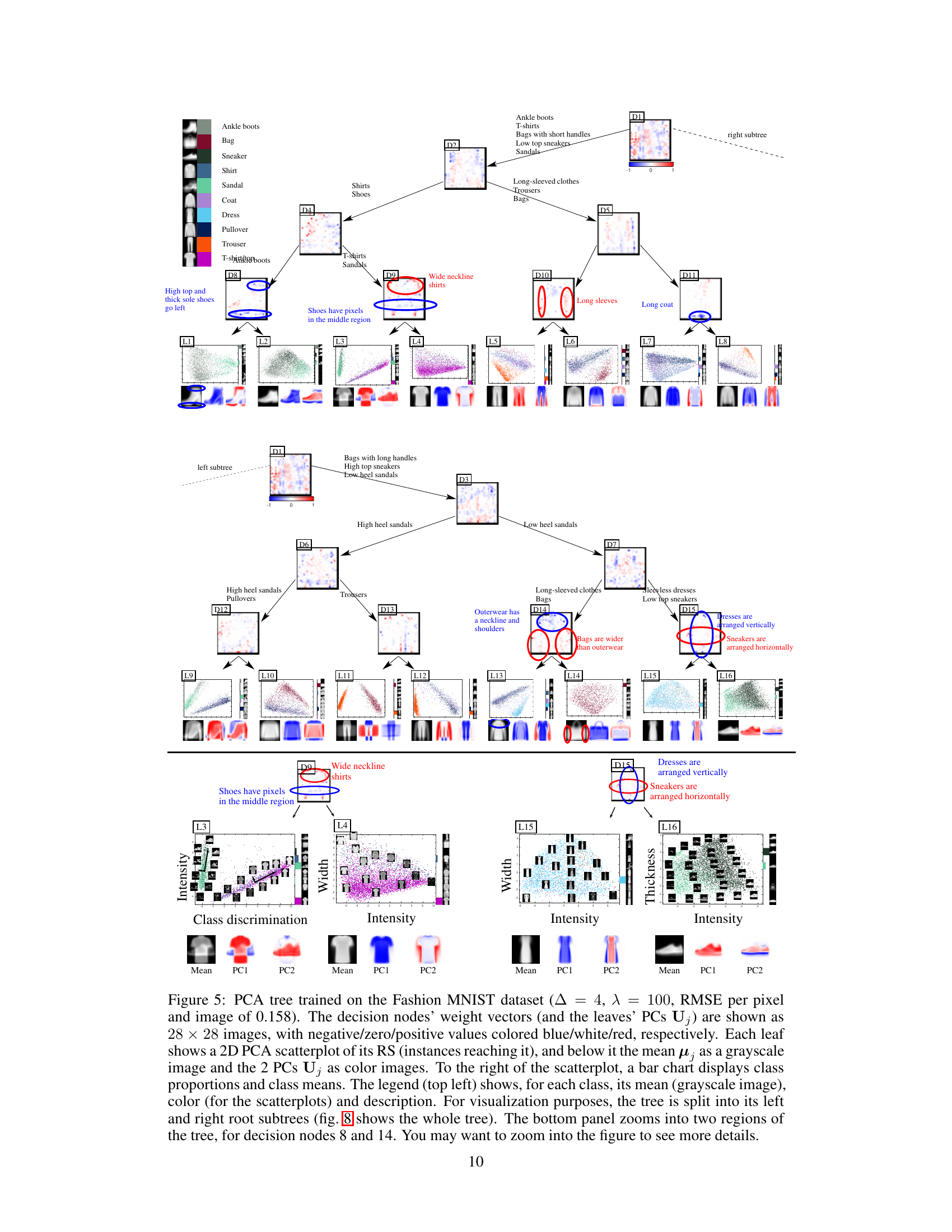
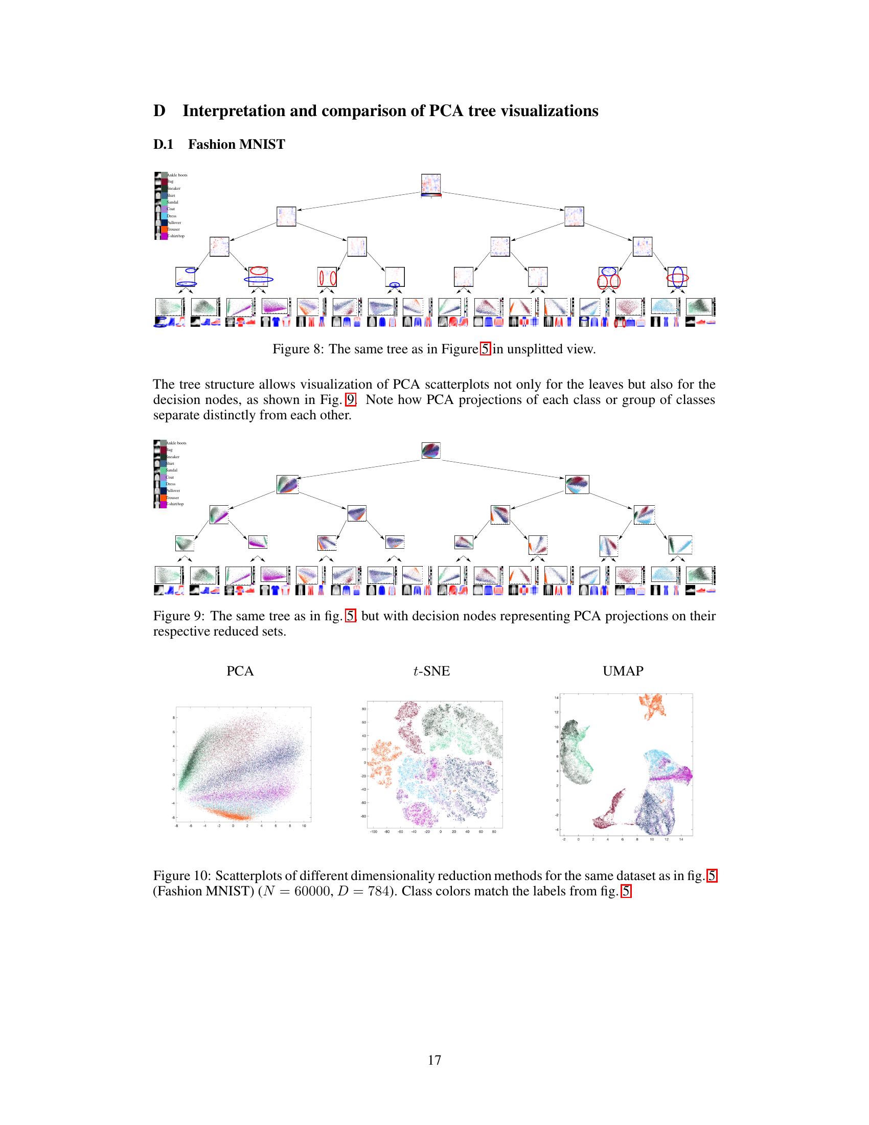
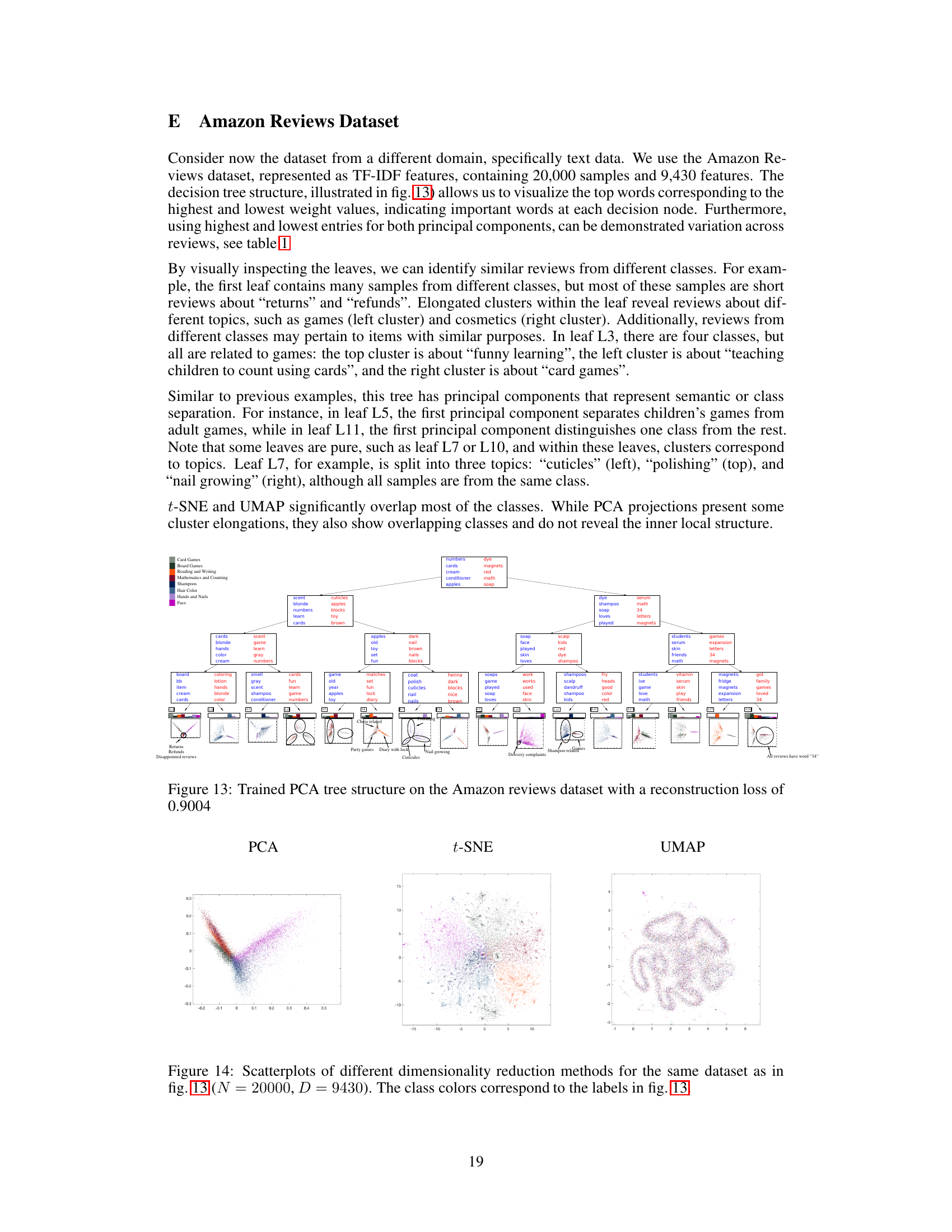
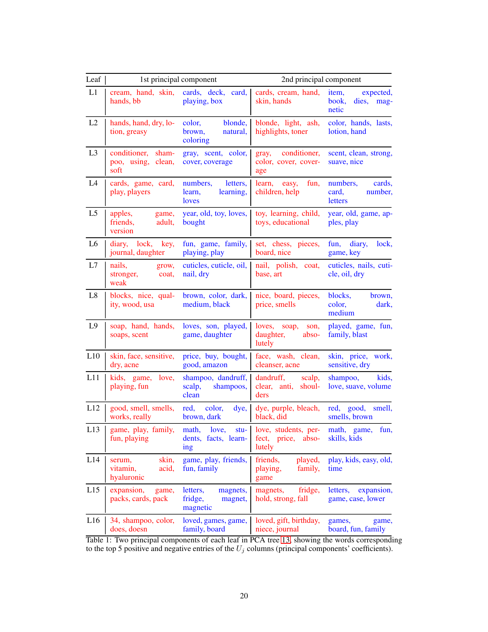
This figure shows a PCA tree trained on the Fashion MNIST dataset. It illustrates the hierarchical structure of the model, where each decision node represents a split based on a subset of features (visualized as 28x28 images), and each leaf node contains a 2D PCA projection of the data points that reach that leaf. The figure visualizes the weight vectors, PCA scatterplots, means, and principal components for each node, providing insights into how the model separates and represents different classes of clothing items.

The pseudocode describes the PCA tree optimization algorithm. It starts with an input training set and hyperparameters. It initializes a tree structure and iteratively refines it by performing PCA on leaf nodes and fitting a regularized binary classifier on decision nodes. This process continues until a stopping criterion is met. The algorithm employs parallelization (parfor) for efficiency, updating each node’s reduced set (instances that reach that node) after each iteration.

This figure displays the objective function values across various training iterations for five different datasets: MNIST, Fashion MNIST, Letter, 20newsgroups, and Amazon Reviews. Each dataset is represented by multiple lines, each corresponding to a different tree depth (∆). The x-axis represents the iteration number, and the y-axis represents the objective function value. The figure demonstrates the monotonic decrease of the objective function during training for all datasets and tree depths, indicating the effectiveness of the proposed optimization algorithm.

This figure shows a PCA tree trained on the Fashion MNIST dataset. It displays the tree structure, with decision nodes represented by 28x28 images showing the feature weights and leaf nodes showing 2D PCA scatterplots of the data points reaching that leaf. The color of the pixels in the decision node images correspond to the weights (blue for negative, white for zero, and red for positive), and the leaf node scatterplots show the data points colored according to their class label. The image also shows the mean and principal components of each leaf.

This figure shows a visualization of a PCA tree trained on the Fashion MNIST dataset. It displays the tree structure, with decision nodes represented by 28x28 images showing the weights and leaves showing 2D PCA scatterplots of their respective regions. Each leaf also includes the mean and principal components as images, along with a bar chart showing class proportions. The figure illustrates how the tree hierarchically separates different classes of clothing items based on visual features. The bottom portion zooms in on two sections to highlight details.
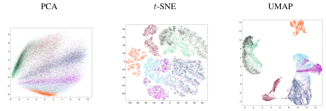
This figure compares the visualization results of three different dimensionality reduction methods: PCA, t-SNE, and UMAP. All three methods were applied to the same Fashion MNIST dataset, which contains 60,000 images of 28x28 pixels (784 features). The color of each point in the scatterplots represents its class label. PCA shows a clear linear separation of some classes, while t-SNE and UMAP show more complex, non-linear structure with varying degrees of cluster separation and distortion. The figure highlights the differences in how each method captures and represents the data’s underlying structure.

This figure shows a trained PCA tree structure on the MNIST dataset, which is a classic dataset of handwritten digits. The tree’s structure is visualized, with each node representing a decision point in the classification process. The leaves of the tree show the final classification results with a reconstruction loss of 0.29. Each node contains a visualization of the data at that point in the tree. The visualization allows one to interpret the decisions made by the tree at various levels. This visual representation makes it easier to understand how the hierarchical structure of the PCA tree achieves dimensionality reduction.
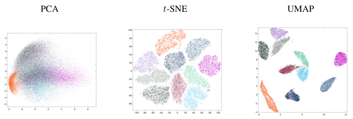
This figure compares the visualizations obtained by PCA, t-SNE, and UMAP on the Fashion MNIST dataset. It highlights the differences in how these methods represent the data’s structure in a two-dimensional space. PCA shows a spread of data points where some class separation is visible, whereas t-SNE arranges the data in a circular fashion with better class separation, while UMAP clusters the data in a more scattered manner with some overlap between classes. The figure illustrates the strengths and weaknesses of each method for dimensionality reduction and visualization.

This figure illustrates a PCA tree trained on the Fashion MNIST dataset. It visualizes the tree structure, showing decision nodes (with their weight vectors as 28x28 images) and leaf nodes (with 2D PCA scatterplots, means, and principal components). The visualization helps interpret how the tree separates different classes hierarchically, revealing meaningful features and low-dimensional structures within each leaf.
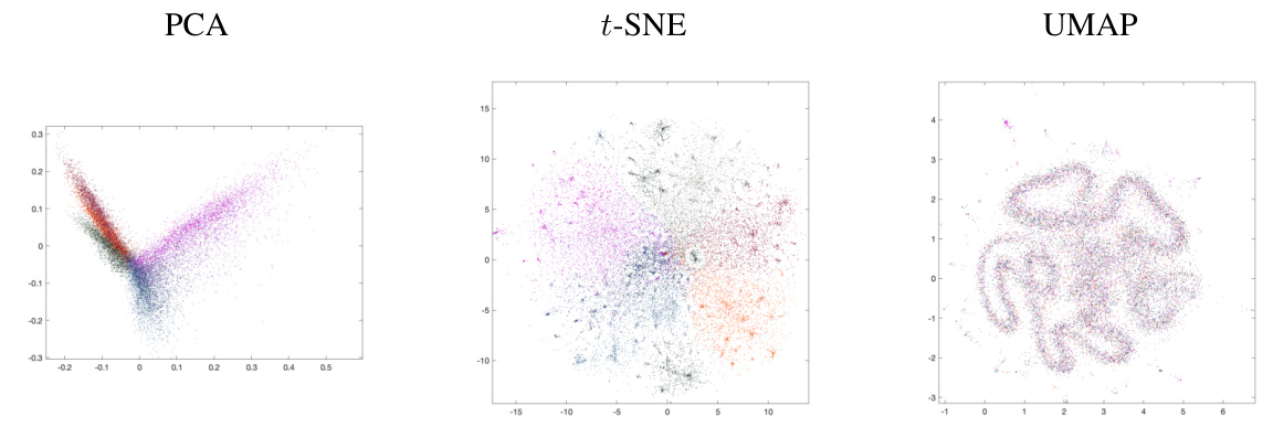
This figure compares the visualization results of three different dimensionality reduction methods: PCA, t-SNE, and UMAP. All three methods were applied to the MNIST dataset (60,000 samples, 784 dimensions), aiming to reduce the data to two dimensions for visualization. The plot shows that PCA preserves the linear structure and clusters better than t-SNE and UMAP, however t-SNE and UMAP visually separate different classes more distinctly. The color of each point indicates the corresponding digit class.
Full paper#
