↗ OpenReview ↗ NeurIPS Homepage ↗ Hugging Face ↗ Chat
TL;DR#
Many real-world applications of partial differential equations (PDEs) suffer from incomplete data. Traditional methods struggle with these scenarios, hindering accurate predictions and estimations. Learning-based solvers offer some improvement, but still require complete information, limiting their applicability.
The paper introduces DiffusionPDE, a generative model-based framework that addresses these limitations. By modeling the joint distribution of PDE coefficients and solutions, DiffusionPDE can effectively manage uncertainty and reconstruct missing information. Experiments on various PDE types demonstrate DiffusionPDE’s superior performance, especially in scenarios with highly sparse data, significantly outperforming existing techniques. This shows a new and versatile approach to PDE solving.
Key Takeaways#
Why does it matter?#
This paper is crucial because it presents a novel framework for solving partial differential equations (PDEs) even when data is incomplete. This is a common challenge in real-world applications where obtaining complete information is often difficult or impossible. The approach offers significant improvements over existing methods, opening avenues for diverse applications and further research.
Visual Insights#
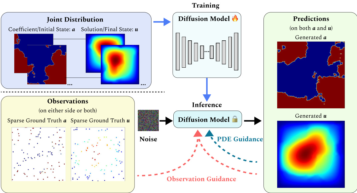
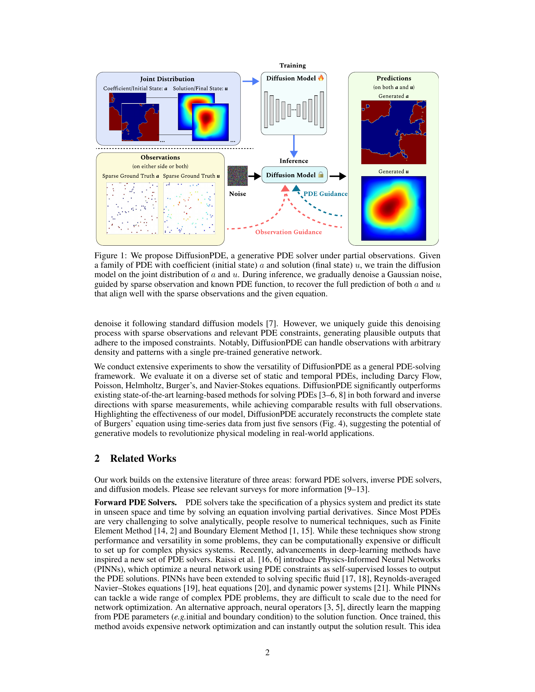
This figure illustrates the architecture of DiffusionPDE, a generative model for solving partial differential equations (PDEs) with partial observations. The training phase involves learning the joint distribution of PDE coefficients (initial state) and solutions (final state) using a diffusion model. During inference, the model takes sparse observations and the known PDE function as input. It then iteratively denoises Gaussian noise, guided by both the sparse observations and the PDE constraints, to reconstruct the full coefficient and solution fields.
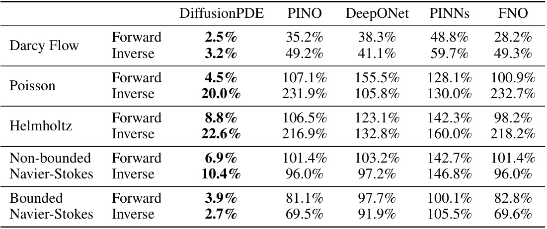
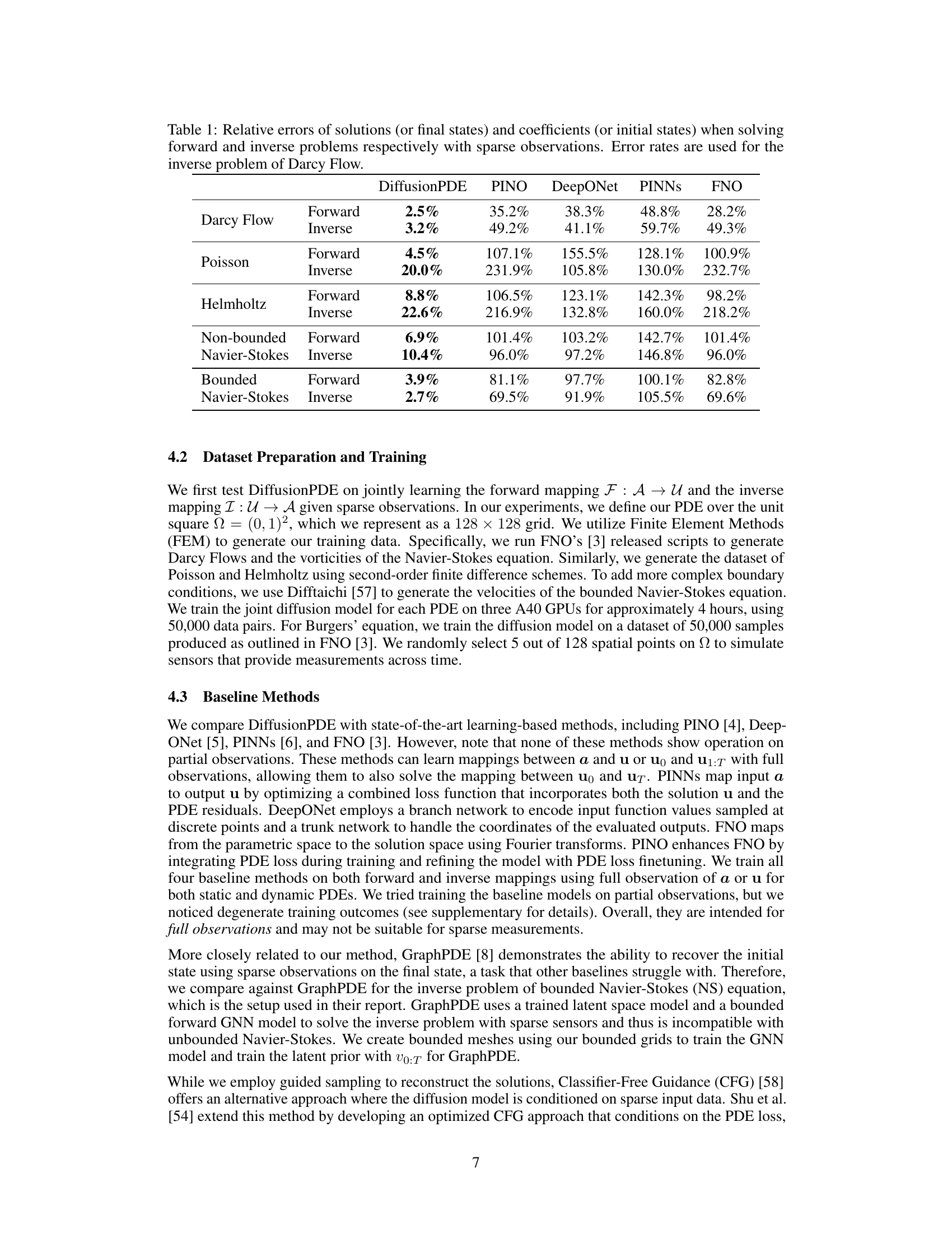
This table presents the relative errors achieved by DiffusionPDE and other state-of-the-art methods (PINO, DeepONet, PINNs, FNO) when solving both forward and inverse problems for various PDEs under sparse observation conditions (typically just 1-3% of total information). The ‘Forward’ column shows the relative error in predicting the solution given sparse observations of the coefficients (or initial states), while the ‘Inverse’ column shows the error in recovering the coefficients given sparse observations of the solution (or final states). For Darcy Flow, the table shows error rates instead of relative errors.
In-depth insights#
DiffusionPDE Framework#
The DiffusionPDE framework presents a novel approach to solving partial differential equations (PDEs) by leveraging the power of generative diffusion models. Its core innovation lies in addressing the challenge of incomplete observations, a common scenario in real-world applications where complete data is rarely available. Instead of relying solely on deterministic mappings, DiffusionPDE models the joint probability distribution of both the PDE coefficients and solutions, enabling simultaneous reconstruction and solving of PDEs under uncertainty. This generative approach allows for the effective management of uncertainty inherent in partial observations and offers a more robust and versatile solution compared to traditional and existing learning-based methods. DiffusionPDE’s ability to handle both forward and inverse problems with high accuracy, even with highly sparse observations, is a significant advancement. Further enhancements such as the integration of PDE guidance during the denoising process enhance accuracy and stability. The framework demonstrates strong potential for diverse applications in scientific computing and related fields.
Guided Diffusion Sampling#
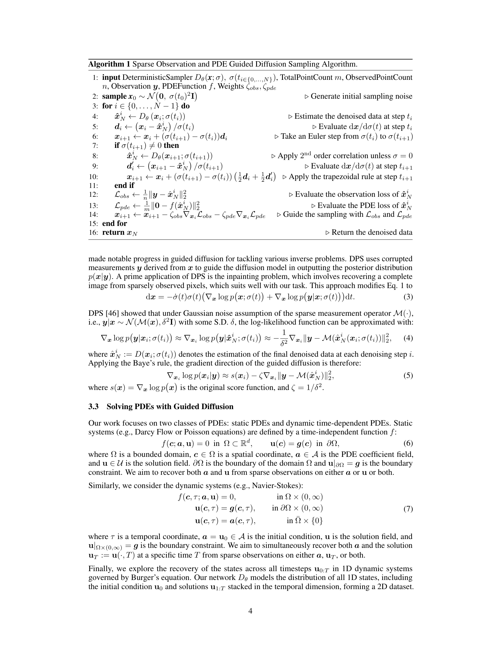
Guided diffusion sampling is a powerful technique that enhances the capabilities of standard diffusion models by incorporating guidance signals during the denoising process. This allows for generating outputs that adhere to specific constraints or desired properties, making it particularly suitable for tasks involving inverse problems or constrained generation. The core idea lies in modifying the standard diffusion process, which iteratively removes noise from a random input to reveal a sample from the target distribution. Instead of purely relying on the learned denoising process, guided diffusion methods add guidance gradients derived from constraints, such as sparse observations in an image inpainting task, or PDE constraints in solving PDEs. This incorporation of guidance steers the denoising process towards outputs conforming to these additional constraints. The method’s effectiveness stems from its ability to balance generative capabilities with the need to satisfy constraints, which enables a versatile approach for complex tasks. By carefully designing the guidance signals and weighting factors, one can effectively control the degree of influence from the guidance, creating a trade-off between fidelity to the constraints and the inherent stochasticity of the diffusion process. A key benefit of guided diffusion models is their capability to manage uncertainty when dealing with incomplete data. By embedding constraints, the denoising process is regularized, leading to more plausible outputs, even under conditions of high uncertainty. This is especially valuable for inverse problems, where obtaining complete observations is often unrealistic. Overall, guided diffusion sampling presents a significant advancement by combining generative models’ strengths with constrained optimization techniques.
PDE Loss Advantage#
The effectiveness of incorporating PDE loss as a guidance mechanism during the denoising process is a pivotal aspect of the research. Adding PDE loss significantly improves the accuracy of the model’s predictions, especially when dealing with sparse observations. This enhancement is observed across a variety of PDE types. The results show that using only observation loss leads to higher errors, indicating that the physical constraints encoded within the PDE are essential for accurate solution reconstruction. The combined guidance of both PDE and observation losses guides the denoising process towards solutions that are both consistent with the available data and satisfy the underlying physical laws governing the PDE, leading to a substantial reduction in error. This finding highlights the crucial role of physics-informed priors in effectively solving PDEs from limited observations. The improvements demonstrate the power of integrating physical knowledge within a generative framework, overcoming the inherent challenges of data sparsity in real-world applications.
Sparse Data Handling#
The effective handling of sparse data is a critical aspect of this research, as it directly addresses the limitations of traditional PDE solvers that struggle with incomplete information. The paper introduces a novel generative approach, DiffusionPDE, to tackle this challenge. Instead of directly estimating solutions from sparse measurements, DiffusionPDE cleverly models the joint probability distribution of both solution and coefficient spaces. This enables it to effectively manage the uncertainty inherent in sparse data, simultaneously reconstructing both the missing information and the solution to the PDE. This strategy shows significant performance gains, especially compared to other learning-based methods that either assume complete observations or struggle with incomplete input. The methodology employs a diffusion model that iteratively denoises Gaussian noise, guided by both sparse measurements and PDE constraints, making the approach flexible and versatile. The impressive results demonstrate DiffusionPDE’s capability to handle various PDE types and diverse sparsity patterns, highlighting the power of generative models for robust and efficient PDE solving in the context of incomplete observations.
Future Research#
The paper’s ‘Future Research’ section would ideally delve into several key areas. First, it should address the limitations of handling only slices of 2D dynamic PDEs, suggesting the need for extending the approach to encompass full temporal intervals. This expansion is crucial for practical applicability. Second, the model’s current struggle with accuracy in constraint-deficient spaces requires investigation. Strategies for improving robustness and accuracy in such scenarios are essential. Third, the relatively slow sampling procedure presents a significant hurdle. Exploring methods to accelerate inference without compromising accuracy is a high priority. Finally, the exploration of different types of PDEs and various types of sparse observations beyond the ones currently tested should be a core focus. Investigating the sensitivity to noise levels and different sampling patterns to enhance robustness and generalizability will further solidify the model’s value. Addressing these points will significantly improve the framework’s potential.
More visual insights#
More on figures

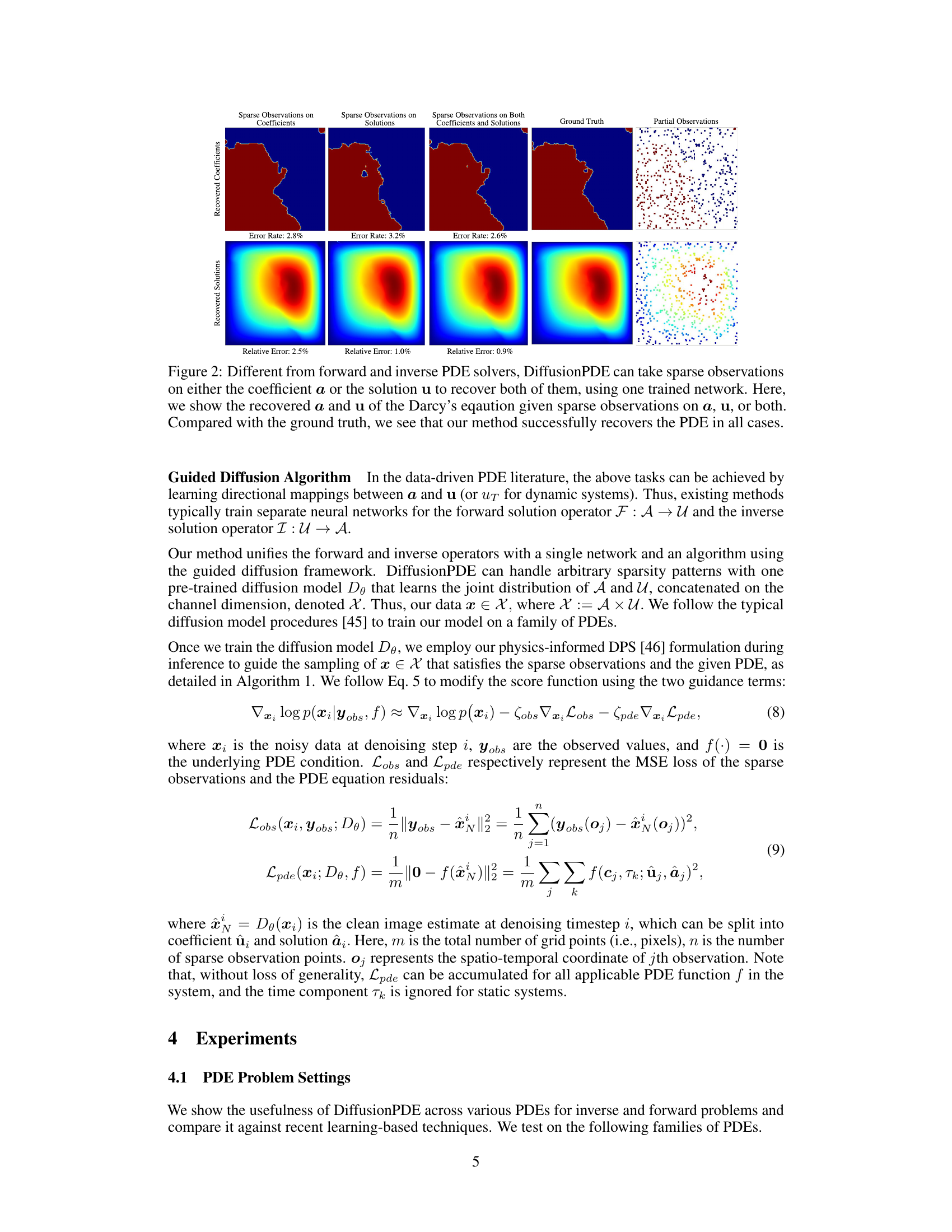
This figure demonstrates the ability of DiffusionPDE to recover both the coefficient and solution of a PDE from sparse observations. It shows three scenarios: sparse observations on the coefficient only, sparse observations on the solution only, and sparse observations on both. Each scenario displays the ground truth coefficient and solution, the corresponding recovered coefficient and solution by DiffusionPDE, and the location of the sparse observations. The error rates (or relative errors) for the recovered data are provided for each scenario. The result demonstrates the versatility of the method, as it can successfully reconstruct the PDE regardless of where the observations come from.

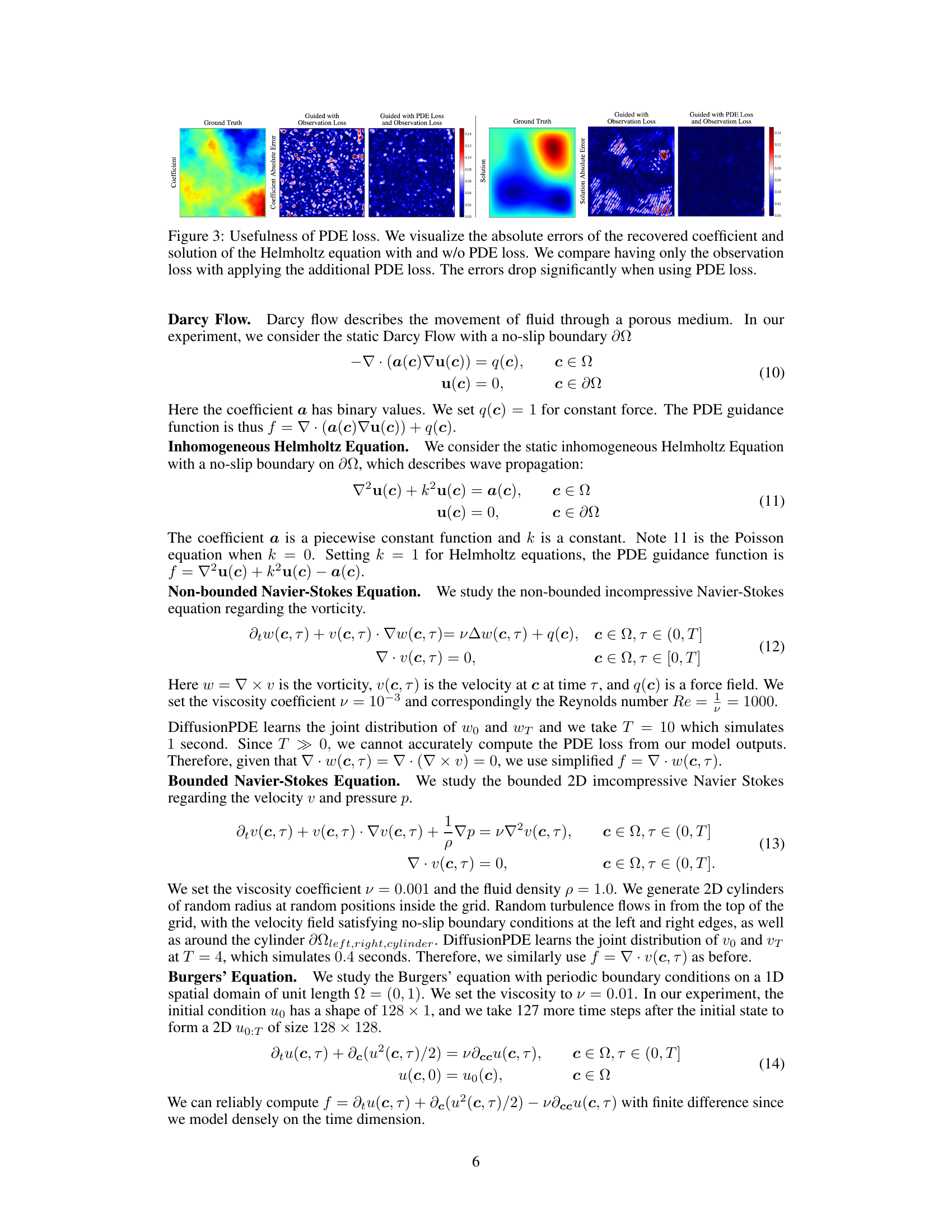
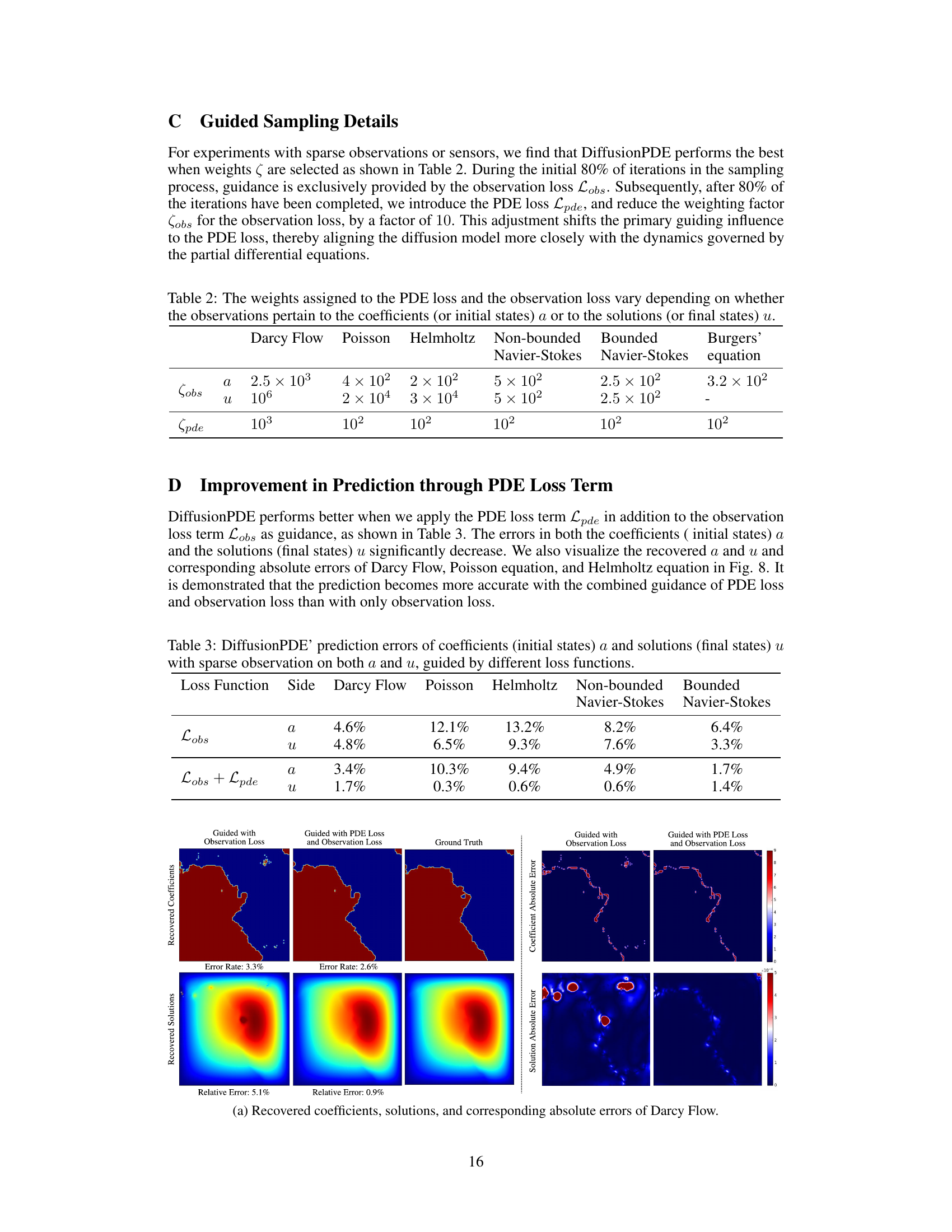
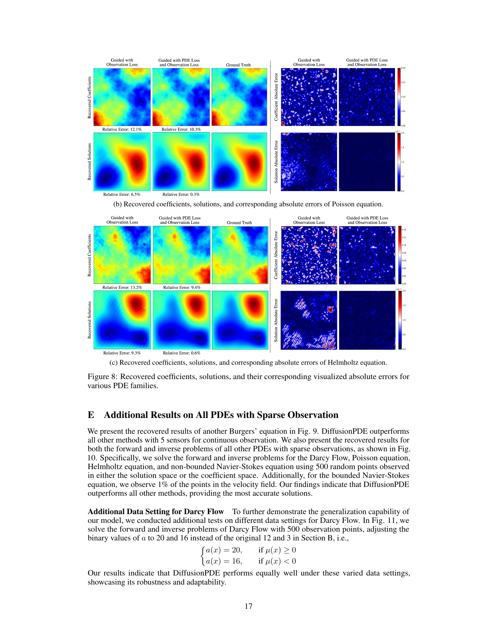
This figure visualizes the results of applying DiffusionPDE to three different types of PDEs: Darcy Flow, Poisson equation, and Helmholtz equation. For each PDE, it shows the ground truth coefficients and solutions alongside the results obtained using DiffusionPDE guided by observation loss only and those obtained using DiffusionPDE guided by both observation and PDE loss. The absolute errors for both coefficients and solutions are also shown in heatmap visualizations, making it clear how the combined use of observation and PDE loss leads to significantly improved accuracy.
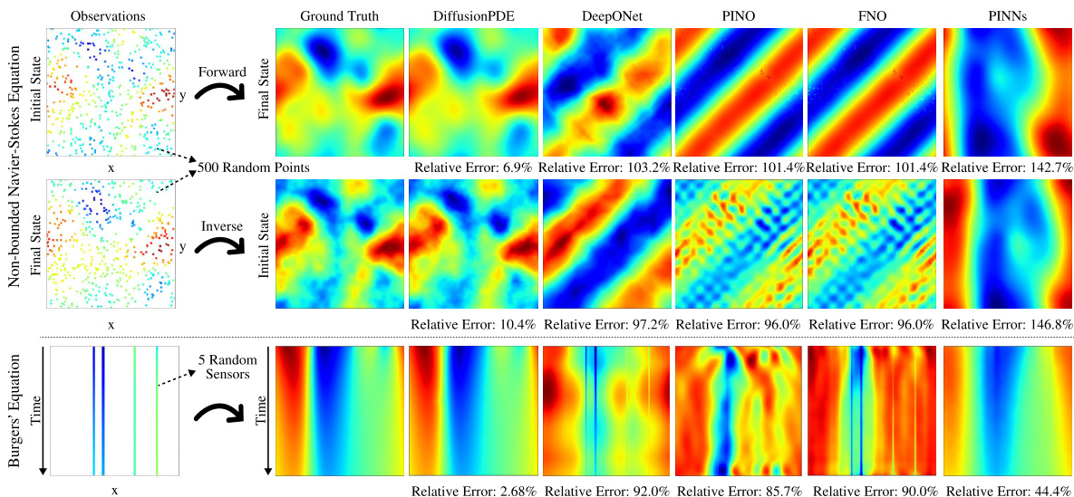
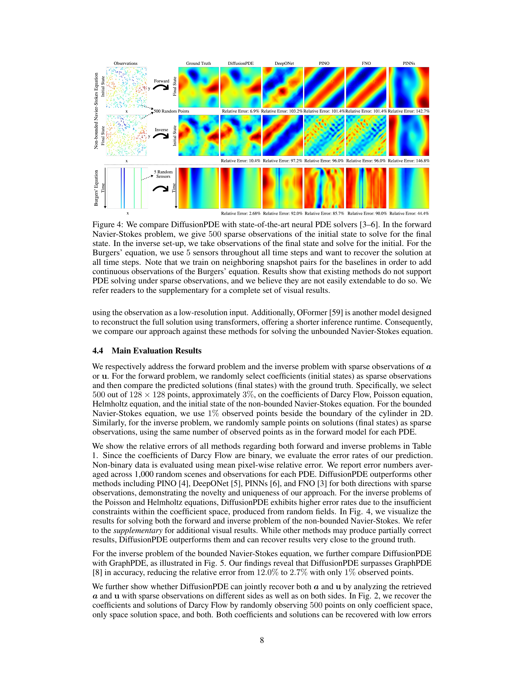
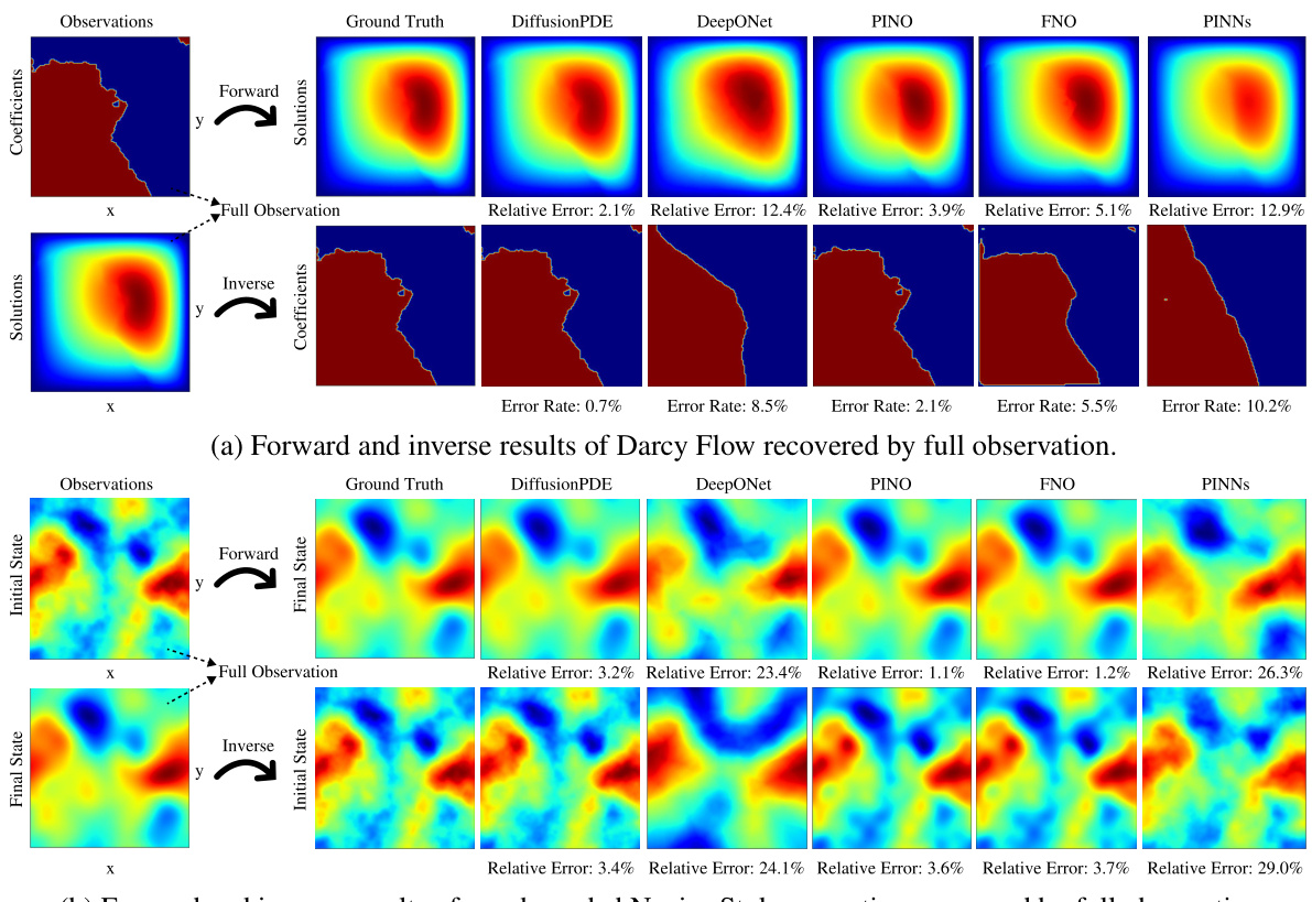
This figure compares the performance of DiffusionPDE against other state-of-the-art neural PDE solvers (DeepONet, PINO, FNO, PINNs) on three different PDE problems: forward and inverse Navier-Stokes and Burgers’ equation. The key takeaway is that DiffusionPDE significantly outperforms the baselines, especially when dealing with sparse observations. While the baselines struggle with even moderately sparse data, DiffusionPDE accurately reconstructs solutions with only a small percentage of observations, showcasing its robustness and effectiveness in handling real-world scenarios where full information is rarely available.

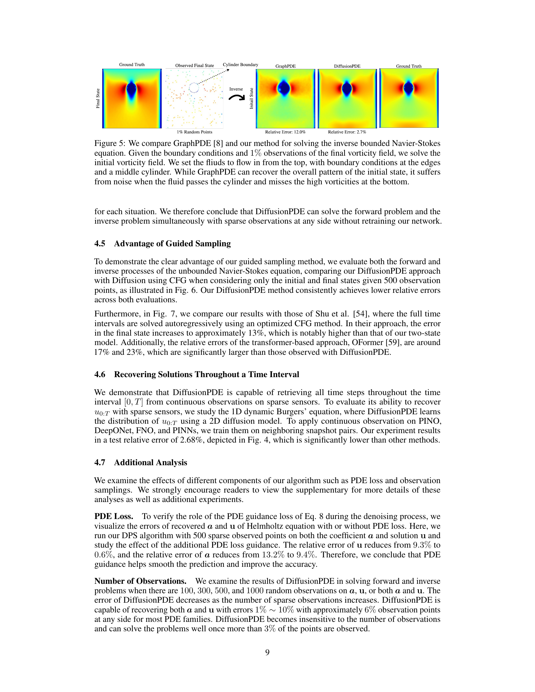
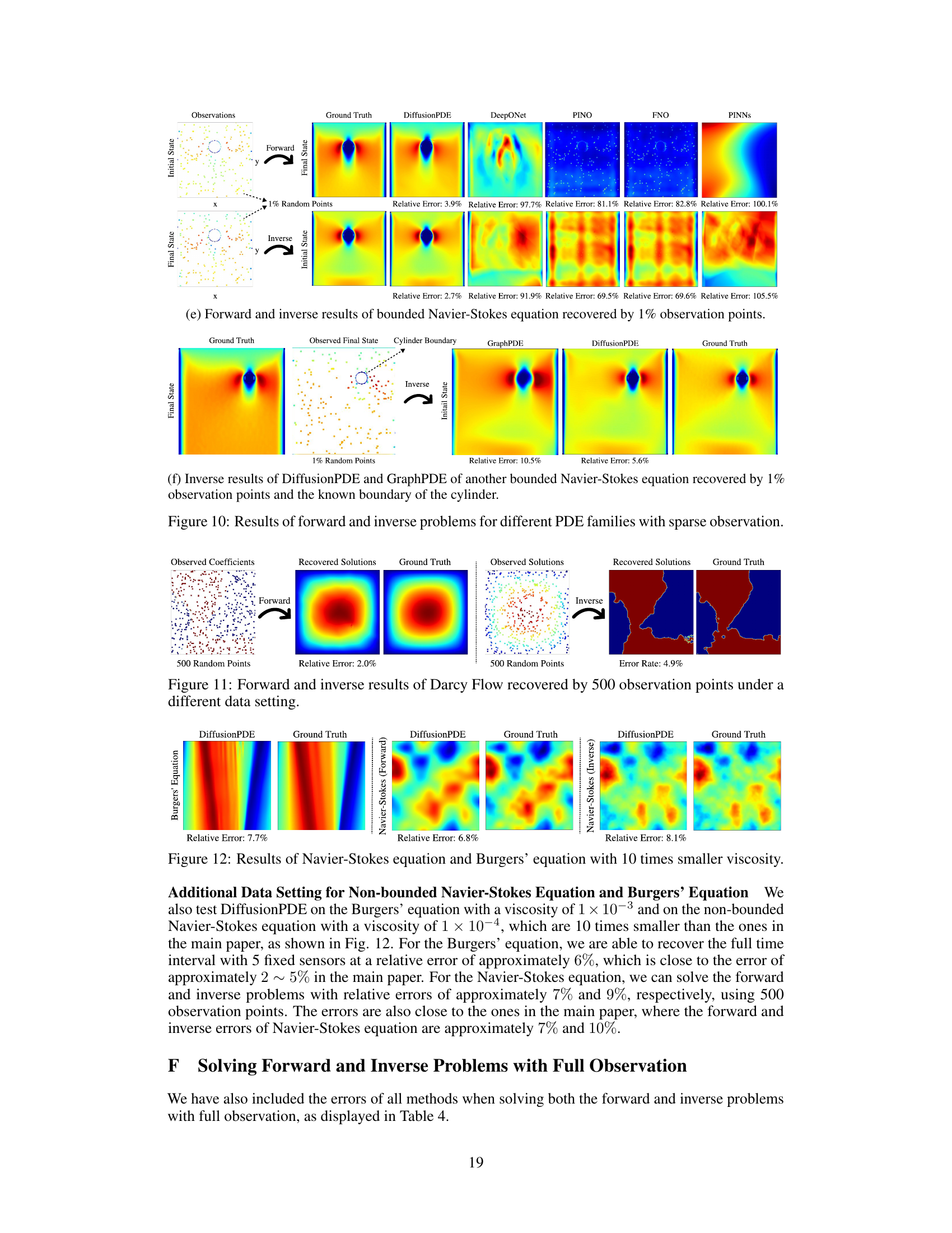
This figure compares the performance of GraphPDE and DiffusionPDE in solving the inverse problem of the bounded Navier-Stokes equation. Both methods are given boundary conditions and 1% of the final vorticity field as input, and are tasked with reconstructing the initial vorticity field. The figure highlights that DiffusionPDE significantly outperforms GraphPDE in accuracy, with a relative error of 2.7% compared to GraphPDE’s 12.0%. The visual representation demonstrates that while GraphPDE recovers the overall shape, it struggles with fine details, particularly around the cylinder. DiffusionPDE produces a much more accurate and detailed reconstruction.
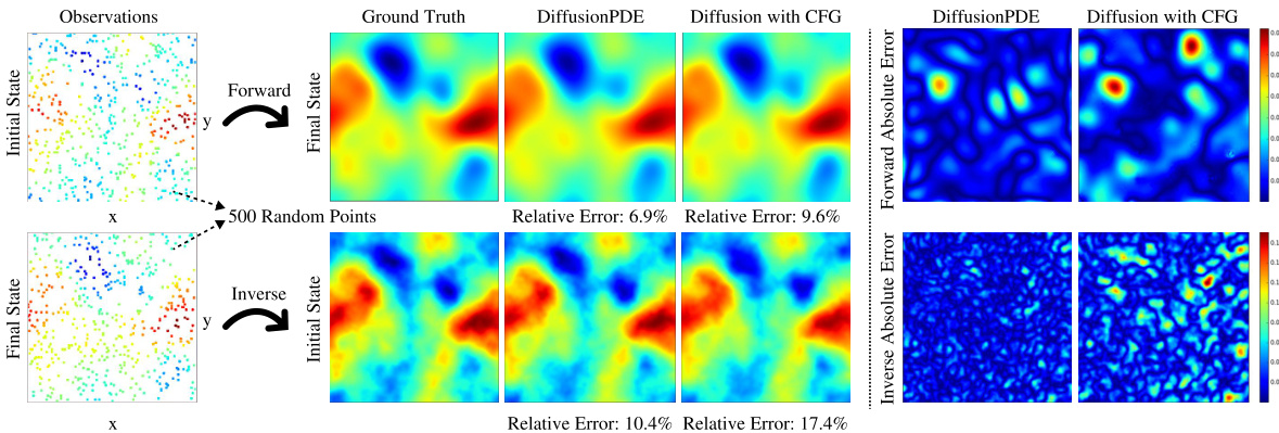
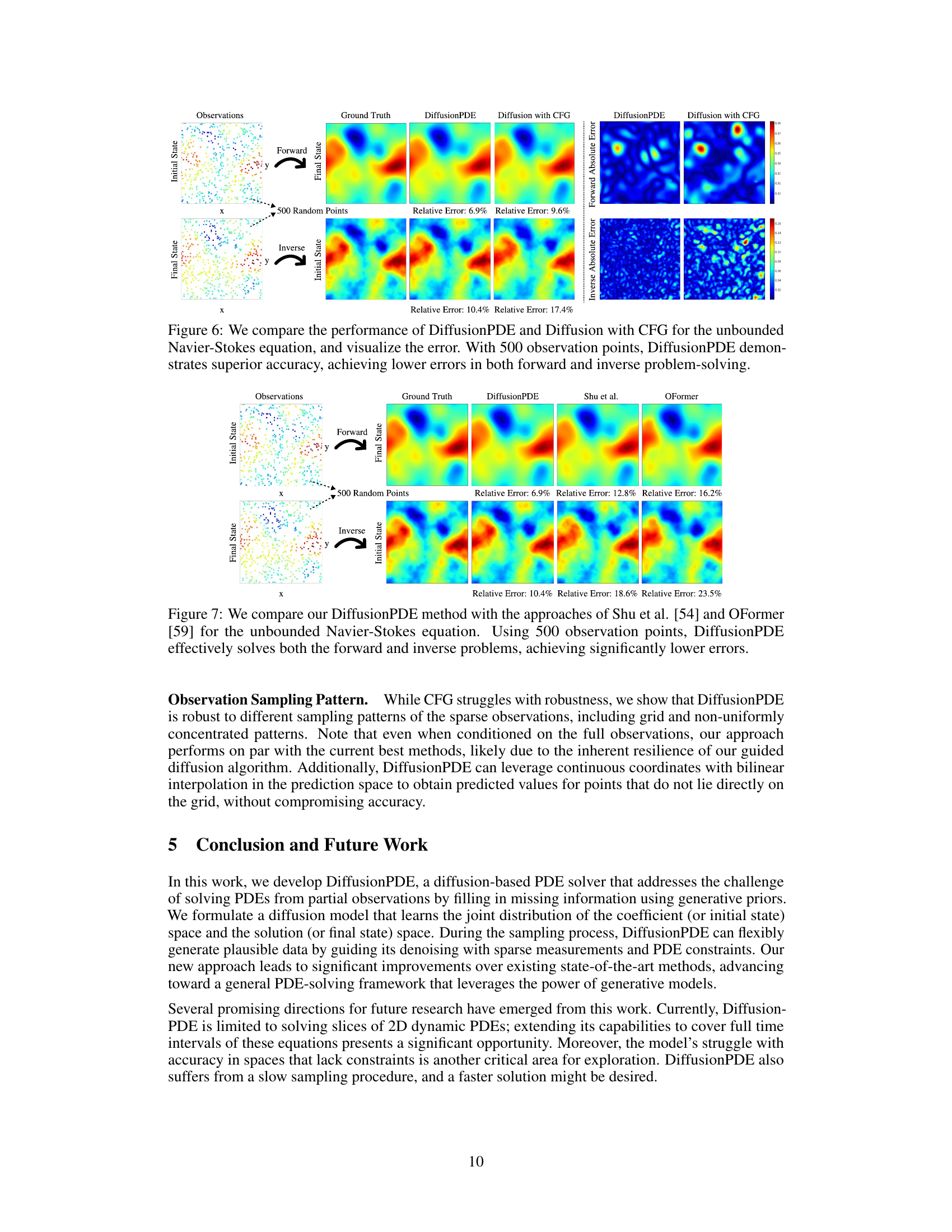
This figure compares the performance of DiffusionPDE and a standard diffusion model with classifier-free guidance (CFG) on the unbounded Navier-Stokes equation. Both methods were given 500 sparse observations (3% of the total data) for solving both the forward and inverse problems. The results demonstrate that DiffusionPDE achieves significantly lower relative errors in both cases, highlighting its superior accuracy for solving PDEs with partial observations.
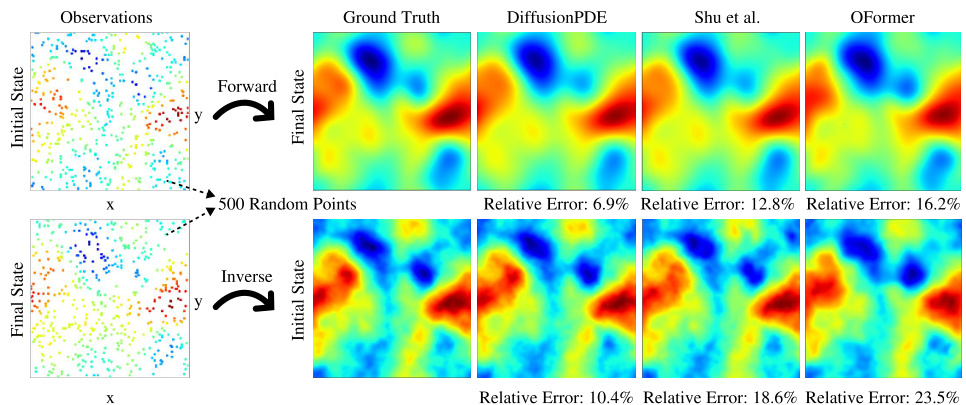
This figure compares the performance of DiffusionPDE against two other methods (Shu et al. and OFormer) on the unbounded Navier-Stokes equation, a complex fluid dynamics problem. The experiment uses 500 sparse observations (only a small percentage of the total data) to solve both the forward problem (predicting the final state from the initial state) and the inverse problem (predicting the initial state from the final state). The results show that DiffusionPDE significantly outperforms the other two methods in terms of accuracy, achieving much lower relative errors.
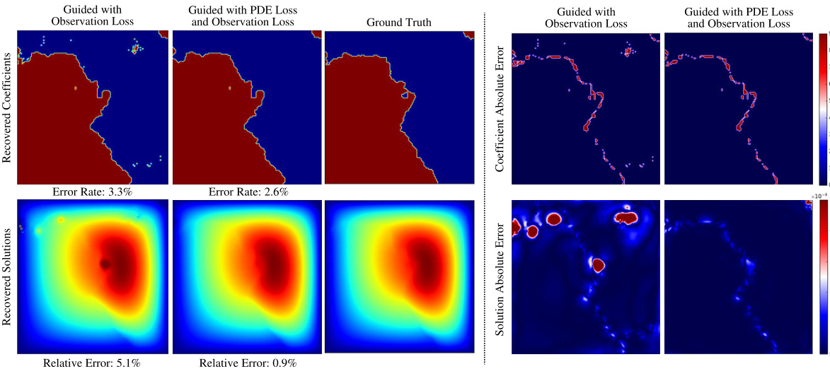
This figure shows the effectiveness of adding PDE loss to the observation loss for improving the accuracy of recovered solutions and coefficients. It visualizes the recovered coefficients, solutions, and corresponding absolute errors for Darcy flow, Poisson equation, and Helmholtz equation, demonstrating the significant improvement in accuracy when both losses are combined.

This figure visualizes the results of DiffusionPDE on three different PDEs: Darcy Flow, Poisson equation, and Helmholtz equation. It shows the recovered coefficients and solutions alongside the ground truth for each PDE. For each PDE, there are three columns representing the results obtained using only observation loss, the combined guidance of observation and PDE loss, and the ground truth. This comparison visually demonstrates the improvement in accuracy achieved by incorporating the PDE loss term in the guidance process. The absolute errors are also visualized, further highlighting the effectiveness of using both the observation and PDE loss.

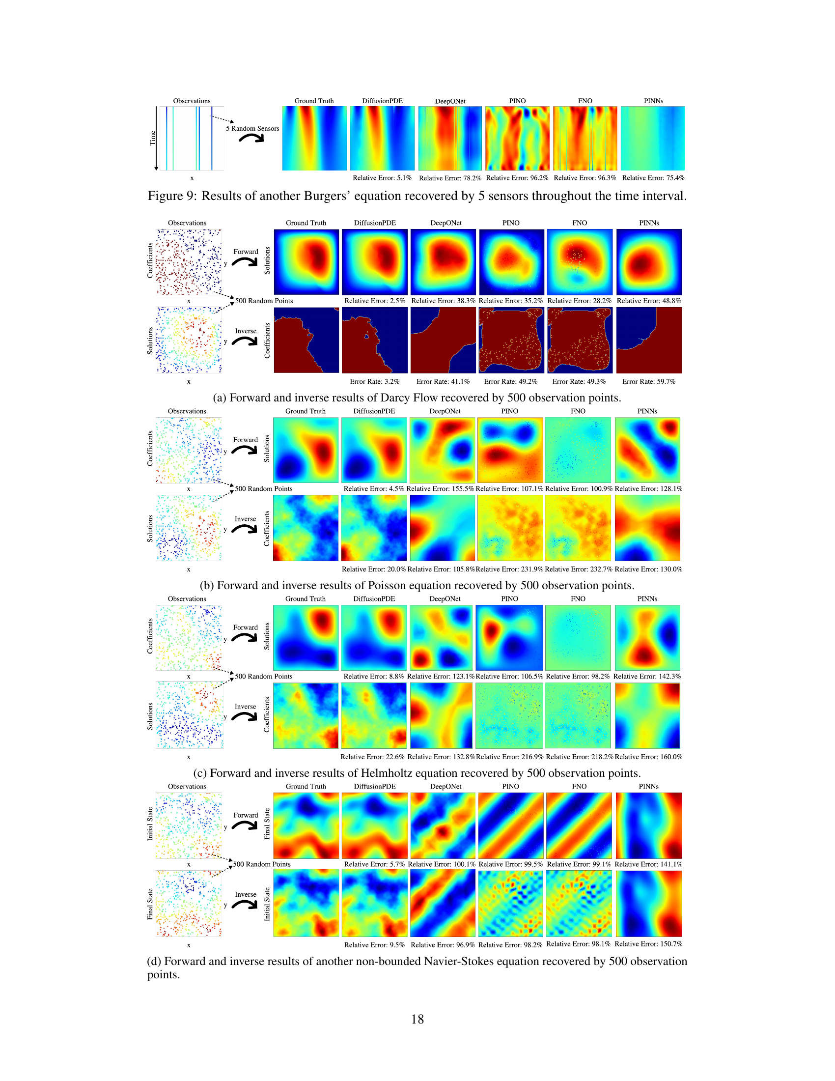
This figure compares the performance of DiffusionPDE against other state-of-the-art neural PDE solvers (DeepONet, PINO, FNO, PINNs) on three different PDE problems (Burgers’, forward Navier-Stokes, and inverse Navier-Stokes). It highlights DiffusionPDE’s ability to accurately solve these problems using significantly fewer observations (5 sensors for Burgers’, 500 sparse observations for Navier-Stokes), showcasing its superior performance under partial observation conditions.

This figure shows the results of DiffusionPDE applied to Darcy’s equation, demonstrating its ability to recover both the coefficient and solution from sparse observations. Three scenarios are presented: sparse observations on the coefficient only, sparse observations on the solution only, and sparse observations on both. The results demonstrate DiffusionPDE’s accuracy compared to the ground truth in all cases. The figure illustrates the versatility of the approach, highlighting its effectiveness even with very limited data.

This figure demonstrates the ability of DiffusionPDE to handle sparse observations. It shows the results of solving the Darcy equation using only sparse observations of either the coefficient (a) or the solution (u), or both. DiffusionPDE successfully reconstructs both the coefficient and solution in each case, highlighting its advantage over traditional methods that require complete information.

This figure visualizes the results of applying DiffusionPDE to various PDEs under sparse observation conditions. It shows both forward (predicting the solution given the coefficients) and inverse (recovering the coefficients given the solution) problems. The results are compared against ground truth, demonstrating the accuracy of DiffusionPDE in reconstructing both coefficients and solutions even with limited information. Each subfigure represents a different PDE, showing the ground truth, sparse observations used, and the results produced by DiffusionPDE and other state-of-the-art methods (DeepONet, PINO, FNO, PINNs, GraphPDE). The relative errors are also indicated for each method, highlighting the superior performance of DiffusionPDE.

This figure demonstrates the ability of DiffusionPDE to solve both forward and inverse problems using only sparse observations of either the coefficient (a) or the solution (u), or both. It showcases the model’s capacity to recover both the full coefficient field and the full solution from incomplete input data, highlighting its versatility compared to traditional methods. The results shown are for Darcy’s equation, but the caption indicates the method performs similarly for other PDEs.

This figure demonstrates the capability of DiffusionPDE to handle partial observations. It showcases the successful reconstruction of both coefficients and solutions of the Darcy equation using only sparse observations of either coefficients, solutions, or both. The results highlight the versatility of DiffusionPDE in handling incomplete data, a major challenge for classical and learning-based PDE solvers.

This figure compares the performance of DiffusionPDE and GraphPDE on solving the inverse problem of the bounded Navier-Stokes equation. Both models use only 1% of the total available information (observations of the final vorticity field). DiffusionPDE is shown to recover the initial vorticity field with significantly greater accuracy and less noise than GraphPDE, particularly in regions of high vorticity near the cylinder.

This figure demonstrates DiffusionPDE’s ability to handle sparse observations. It shows results for solving the Darcy’s equation using the proposed method. Three scenarios are presented: sparse observations on the coefficient (a), sparse observations on the solution (u), and sparse observations on both the coefficient and the solution. The figure visually compares the recovered coefficient and solution in each scenario with their ground truth counterparts. The relative error rate is provided for each case, demonstrating the accuracy of the method even with limited information.

This figure compares DiffusionPDE to other state-of-the-art methods for solving PDEs with sparse observations. It shows the results of forward and inverse problems for the Navier-Stokes and Burgers’ equations, highlighting DiffusionPDE’s superior performance, particularly in scenarios with highly limited data (e.g., only 5 sensors for the Burgers’ equation).
This figure illustrates the overall architecture of DiffusionPDE, a generative model for solving partial differential equations (PDEs) when only partial observations are available. The model is trained on the joint distribution of PDE coefficients (initial state) and their corresponding solutions (final state). During inference, the model takes noisy data as input and iteratively denoises it, guided by both sparse observations of the solution or coefficient and the known PDE constraints. The output is a full reconstruction of both the coefficient and solution spaces, consistent with both the observations and the PDE.
This figure shows that DiffusionPDE can handle sparse observations of either the coefficient or the solution to recover both using a single trained network. It demonstrates the results of using DiffusionPDE to solve Darcy’s equation with sparse observations of the coefficient, solution, or both. The results are compared to the ground truth, and the low error rates demonstrate the effectiveness of DiffusionPDE.

This figure demonstrates the ability of DiffusionPDE to recover both the coefficients (a) and solutions (u) of a partial differential equation (PDE), specifically Darcy’s equation, using sparse observations. It showcases three scenarios: sparse observations on coefficients only, sparse observations on solutions only, and sparse observations on both. In each scenario, DiffusionPDE successfully recovers both a and u, which are visually compared to the ground truth, indicating the model’s accuracy even with limited data.
This figure illustrates the architecture of DiffusionPDE, a generative model for solving partial differential equations (PDEs) with only partial observations of the solution and/or coefficients. The model is trained on the joint distribution of the PDE coefficients (initial state) and the corresponding solutions (final state). During inference, the model takes as input a noisy version of the solution and/or coefficients and iteratively denoises it, guided by sparse observations and the known PDE, to recover the complete solution and coefficients.

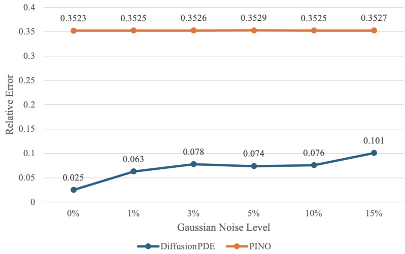
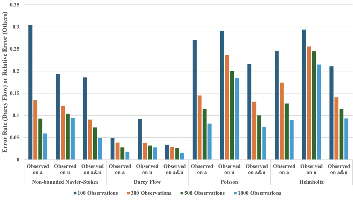
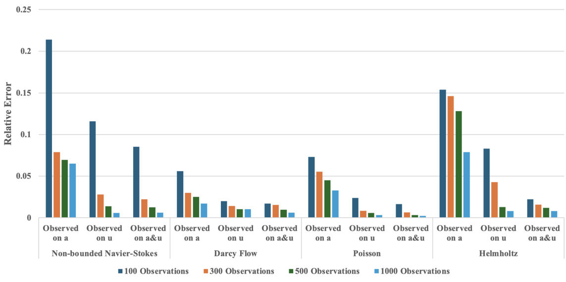
This figure demonstrates the robustness of DiffusionPDE against noisy observations. It shows the relative error of recovered Darcy Flow solutions when different levels of Gaussian noise (0%, 1%, 3%, 5%, 10%, and 15%) are added to the sparse observations. The results indicate that DiffusionPDE maintains relatively low error rates even with a significant amount of noise.

This figure demonstrates the ability of DiffusionPDE to handle sparse observations. It shows three scenarios: sparse observations of only the coefficient (a), only the solution (u), and both a and u. In each scenario, DiffusionPDE successfully reconstructs both the coefficient and the solution of the Darcy equation, showcasing its effectiveness even with highly incomplete data.

This figure compares the performance of the proposed DiffusionPDE method and a standard diffusion model using classifier-free guidance (CFG) on the unbounded Navier-Stokes equation. The experiment uses 500 sparse observations. Both forward (predicting the final state from the initial state) and inverse (predicting the initial state from the final state) problems are evaluated. The figure visually shows the ground truth, DiffusionPDE results, CFG results, and the relative errors of each. DiffusionPDE shows significantly lower errors in both forward and inverse settings.
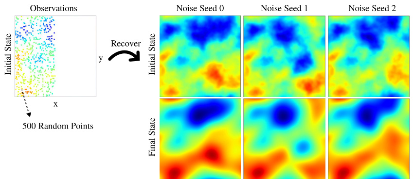
This figure demonstrates the ability of DiffusionPDE to handle sparse observations in solving partial differential equations (PDEs). It shows results for the Darcy equation, where only a small percentage (1-3%) of the total data is available as observations, either for the coefficient ((a)) or the solution ((u)) or both. DiffusionPDE successfully recovers the full coefficient field and solution with high accuracy by using one trained network and sparse observations.
This figure demonstrates the ability of DiffusionPDE to handle sparse observations. It shows the recovered coefficients and solutions for Darcy’s equation when only sparse observations of either the coefficients, solutions, or both are available. The results are compared to the ground truth, highlighting the accuracy of DiffusionPDE even with limited data.
This figure demonstrates the ability of DiffusionPDE to handle sparse observations in both forward and inverse problems. It shows the results of using DiffusionPDE to solve the Darcy equation, given sparse observations of the coefficient (a), solution (u), or both. The recovered coefficients and solutions are compared to the ground truth, showcasing DiffusionPDE’s ability to accurately recover the PDE under partial observations.

This figure demonstrates DiffusionPDE’s ability to handle sparse observations in both forward and inverse PDE solving problems. It shows that DiffusionPDE can recover both the coefficient and solution of the Darcy equation accurately even when only a small percentage of observations are available for either the coefficient or the solution, or both. The results highlight the versatility of DiffusionPDE compared to traditional methods that typically require full observations.

This figure shows the results of applying DiffusionPDE to solve the Darcy equation under three different scenarios of partial observation: sparse observation of coefficient (a), sparse observation of solution (u), and sparse observation of both (a and u). The figure visually compares the recovered coefficients and solutions obtained by DiffusionPDE with the ground truth for each scenario, demonstrating that DiffusionPDE accurately recovers the solution even with limited observations.
More on tables

This table shows the weights used in the DiffusionPDE algorithm for balancing the observation loss and the PDE loss during the sampling process. The weights vary depending on whether the observations are on the coefficients (a) or the solutions (u) and also depend on the specific PDE being solved (Darcy Flow, Poisson, Helmholtz, Non-bounded Navier-Stokes, Bounded Navier-Stokes, and Burgers’ equation). The weights are adjusted to shift the primary guiding influence to the PDE loss after 80% of the sampling iterations.

This table shows the prediction errors of coefficients (initial states) and solutions (final states) achieved by DiffusionPDE using different loss functions. The errors are presented for several types of PDEs (Darcy Flow, Poisson, Helmholtz, Non-bounded Navier-Stokes, and Bounded Navier-Stokes) when using only the observation loss (Lobs) and when combining the observation loss with the PDE loss (Lobs + Lpde). Lower error percentages indicate better performance.
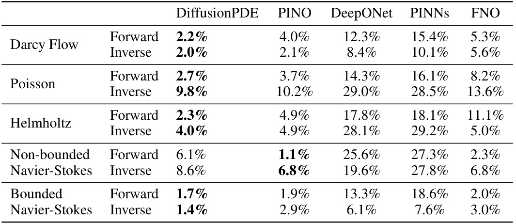
This table presents the relative errors achieved by DiffusionPDE and other state-of-the-art methods (PINO, DeepONet, PINNs, FNO) when solving both forward and inverse PDE problems using sparse observations (typically 1-3%). The relative error measures the accuracy of the predicted solutions (or final states) compared to the ground truth. For the inverse problem of Darcy Flow, error rates are reported instead of relative errors, reflecting the use of binary values for coefficients. The results showcase DiffusionPDE’s superior performance in both forward and inverse problems under partial observation conditions.

This table presents the relative errors achieved by DiffusionPDE and other state-of-the-art methods (PINO, DeepONet, PINNs, and FNO) when solving forward and inverse PDE problems using sparse observations. The relative error measures the difference between the model’s prediction and the ground truth. For the inverse problem of Darcy flow, error rates are provided instead of relative errors. Lower values indicate better performance.

This table presents the performance of DiffusionPDE and several other state-of-the-art methods for solving forward and inverse PDE problems using sparse observations (around 3%). The relative errors in the solutions (or final states, ‘u’) and coefficients (or initial states, ‘a’) are shown for various PDEs, including Darcy flow, Poisson, Helmholtz, and Navier-Stokes equations (both bounded and unbounded). For the inverse problem of Darcy flow, error rates are used instead of relative errors.

This table compares the computational cost of four different methods for solving partial differential equations using sparse observations. The methods compared are DiffusionPDE (the proposed method), GraphPDE, Shu et al. (2023), and OFormer. The metrics used for comparison are the number of parameters (in millions), inference time (in seconds), and GPU memory usage (in gigabytes).

This table presents the relative errors achieved by DiffusionPDE and other baseline methods (PINO, FNO, DeepONet, PINNs) when solving forward and inverse PDE problems using sparse observations. The baseline methods’ results were improved by an optimization process. The table showcases the performance of DiffusionPDE, highlighting its superiority in accuracy, especially when compared to optimized baseline methods.

This table presents the relative errors achieved by DiffusionPDE and other state-of-the-art methods (PINO, DeepONet, PINNs, FNO) when solving forward and inverse PDE problems using sparse observations. For each PDE (Darcy Flow, Poisson, Helmholtz, Non-bounded Navier-Stokes, Bounded Navier-Stokes), the table shows the relative error for both forward and inverse problems, indicating the performance of each method under conditions of limited data. The use of error rates versus relative errors is specified; specifically, error rates are used for the inverse problem of Darcy Flow.
Full paper#
