↗ OpenReview ↗ NeurIPS Homepage ↗ Chat
TL;DR#
Many imaging problems are ill-posed, meaning there are many possible solutions that fit the available data. Posterior sampling aims to find many likely solutions, quantifying uncertainty and improving robustness. Current posterior samplers using cGANs have limitations in accuracy and speed.
pcaGAN improves upon existing cGAN-based posterior samplers by adding a novel regularization method. This regularization ensures that the generated samples accurately reflect not only the posterior mean but also its principal components. Experiments show pcaGAN outperforms other cGANs and diffusion models across various imaging tasks, achieving significantly faster sampling speeds while maintaining or improving accuracy.
Key Takeaways#
Why does it matter?#
This paper is important because it presents pcaGAN, a novel method that significantly improves the accuracy and speed of posterior sampling in conditional generative adversarial networks (cGANs). This addresses a key challenge in ill-posed imaging inverse problems, where obtaining accurate and diverse samples from the posterior distribution is crucial for uncertainty quantification and robust recovery. The method’s superior performance over existing cGANs and diffusion models, particularly its speed advantage, makes it highly relevant to various imaging applications and opens new avenues for research in this field.
Visual Insights#

This figure shows the results of a Gaussian experiment designed to compare the performance of pcaGAN, rcGAN, and NPPC in recovering synthetic Gaussian data. The Wasserstein-2 distance (W2), a metric measuring the difference between the true and estimated posterior distributions, is plotted against three variables: (a) the lazy update period M in pcaGAN, (b) the number of estimated eigen-components K in pcaGAN, and (c) the problem dimension d for all three methods. This experiment helps to assess the impact of various parameters and problem complexities on the accuracy of the algorithms.

This table presents the quantitative results of MNIST denoising experiments. It compares the performance of three different models: NPPC, rcGAN, and pcaGAN (with K=5 and K=10). The metrics used for comparison include root mean squared error (rMSE), residual error magnitude (REM5), conditional Fréchet Inception Distance (CFID), and inference time for 128 images. Lower values for rMSE, REM5, and CFID indicate better performance, while a shorter inference time is also preferred.
In-depth insights#
PCA-GAN’s novelty#
PCA-GAN introduces novelty by regularizing the posterior distribution’s principal components. Unlike prior cGAN approaches focusing solely on mean and covariance trace, PCA-GAN directly targets the K most significant principal components of the posterior covariance matrix, improving the accuracy of the generated samples’ covariance structure. This novel regularization approach leads to more accurate representation of uncertainty and superior performance across various imaging tasks. The incorporation of a lazy regularization strategy further enhances efficiency by reducing computational overhead. The method’s effectiveness in capturing posterior principal components also surpasses that of dedicated NPPC networks, indicating a more holistic and efficient approach to posterior sampling. The combination of regularization on mean, trace, and principal components ensures correctness across multiple key aspects of the posterior distribution, producing samples with improved perceptual quality, speed, and accuracy.
Regularization effects#
Regularization, crucial in training deep generative models like the pcaGAN, prevents overfitting by constraining the model’s complexity. The choice of regularization (e.g., L1, L2, or a custom penalty) significantly impacts performance. In pcaGAN, the authors employ a novel approach by incorporating penalties not only on the posterior mean but also on its principal components and trace-covariance, aiming for a more accurate representation of the posterior distribution. This multi-faceted regularization strategy, compared to simpler methods focusing solely on the mean, is shown to yield superior performance in recovering image data. The benefits observed suggest that correcting the principal components of the posterior covariance matrix is particularly valuable, especially in scenarios with significant uncertainty. Ultimately, the effectiveness of the regularization is demonstrated across diverse image recovery tasks (denoising, inpainting, MRI reconstruction), highlighting its broad applicability and the advantages of going beyond basic mean-based regularization.
Empirical evaluations#
A robust empirical evaluation section is crucial for validating the claims of a research paper. It should go beyond simply presenting results; instead, it needs to demonstrate a clear understanding of the methodology and limitations. Careful selection of metrics is vital; choosing metrics that directly reflect the paper’s goals ensures the evaluation is meaningful. The paper should demonstrate that the chosen approach is superior by presenting comparative results against strong baselines using standard benchmarks where possible. This is important to demonstrate that improvements are significant and not merely incremental. A strong section would also discuss potential confounding factors and limitations and would acknowledge any unexpected results. Transparency about experimental setups and parameters is essential for reproducibility. The discussion of results must connect back to the paper’s introduction and the initial claims made. Ultimately, a thoughtful empirical evaluation establishes the validity and impact of the research.
Computational cost#
A crucial factor in evaluating the practicality of any machine learning model, especially in resource-intensive applications such as medical image processing, is the computational cost. The paper’s focus on speed, particularly in achieving orders-of-magnitude faster posterior sampling than diffusion models, suggests a significant improvement in computational efficiency. This speed advantage is likely due to the algorithmic design of the proposed pcaGAN, which avoids the computationally expensive iterative processes inherent in many diffusion methods. However, the paper does acknowledge that training pcaGAN can still be computationally demanding, especially in high dimensional spaces. The use of lazy regularization and efficient optimization techniques mitigate these costs to some extent, although the specific runtime impacts of these strategies and other details require further scrutiny. Therefore, a thorough analysis should involve quantifying the trade-off between model accuracy and computational cost across various datasets and problem settings. A detailed breakdown of memory requirements and energy consumption would also greatly enhance understanding and offer a truly comprehensive evaluation of the pcaGAN’s real-world applicability.
Future works#
Future work in this research could involve exploring more advanced regularization techniques beyond principal component analysis to further enhance the accuracy and diversity of posterior samples. Investigating alternative GAN architectures or hybrid models combining GANs with other generative methods like diffusion models might also prove fruitful. Extending the methodology to a wider range of inverse problems beyond those considered in the paper is crucial for demonstrating its generalizability and impact. This includes exploring applications in medical imaging modalities beyond MRI and tackling challenges such as handling high-dimensional data more efficiently. Finally, a rigorous uncertainty quantification framework built upon the generated posterior samples could provide a powerful tool for evaluating the reliability of the generated image reconstructions and improving the trust in AI-driven image analysis.
More visual insights#
More on figures

This figure compares the performance of pcaGAN and NPPC on MNIST denoising. For each model, it shows the true image, the noisy measurement, the estimated posterior mean, the top 5 principal eigenvectors, and two reconstructions obtained by adding multiples of the eigenvectors to the posterior mean. This visualization helps to understand how each model captures uncertainty and generates diverse samples from the posterior distribution.
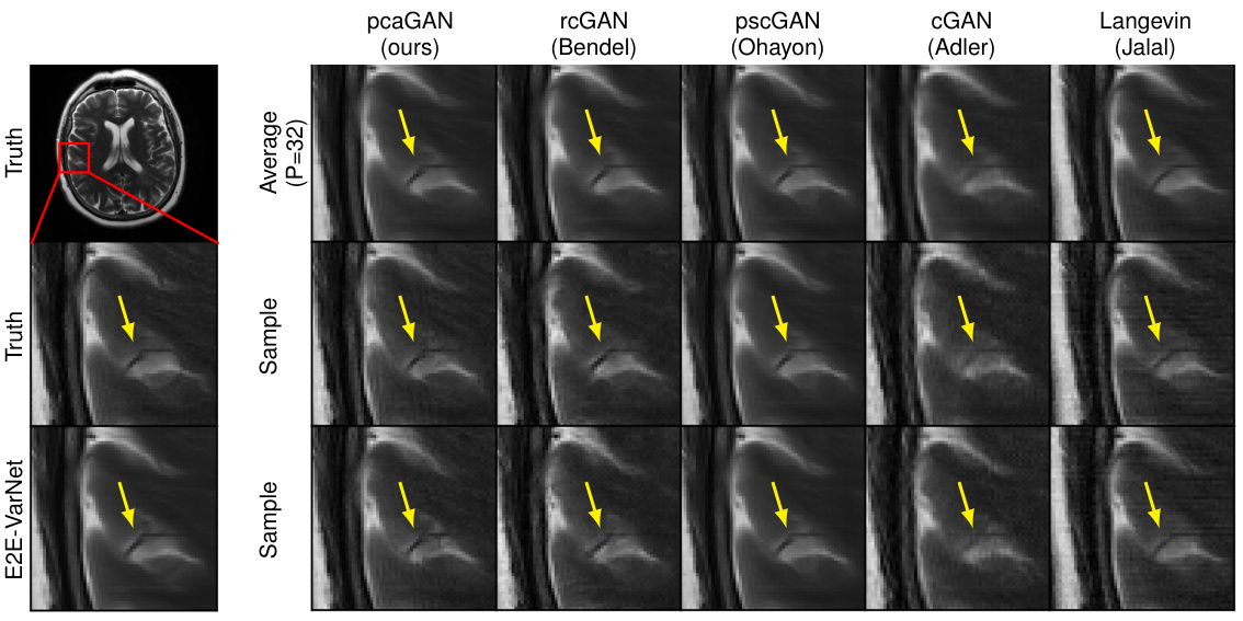
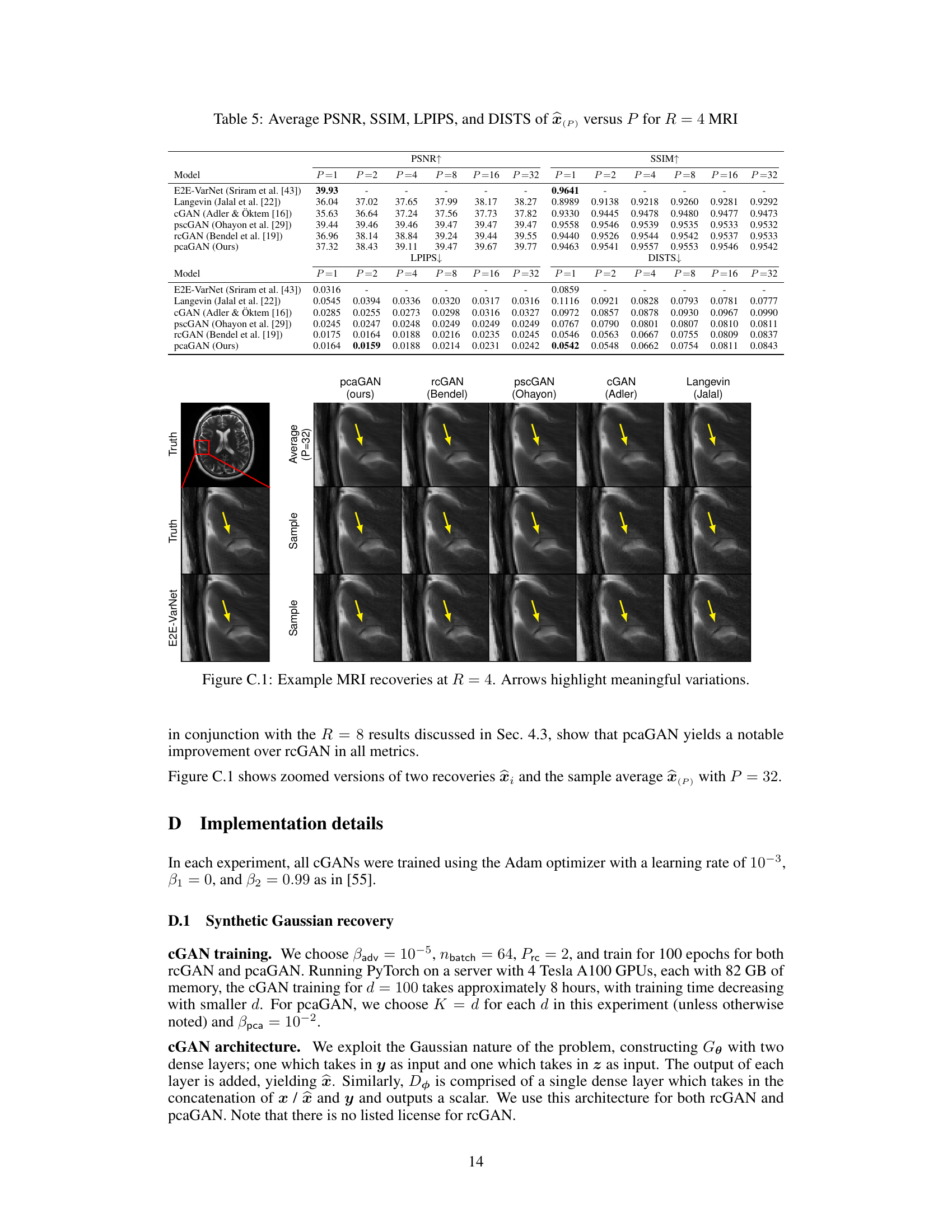
This figure shows the results of MRI recovery at acceleration factor R=8 using different methods. The first row shows the ground truth, followed by the average of 32 samples generated by pcaGAN and other methods such as rcGAN, pscGAN, CGAN, and Langevin. The last row shows samples generated by E2E-VarNet. Arrows highlight variations between the different recovery methods, illustrating the relative performance of each technique.
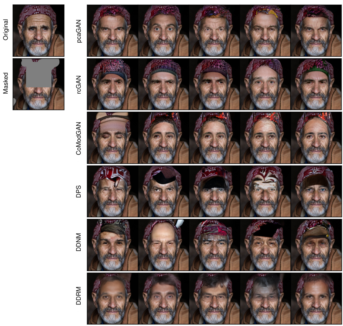
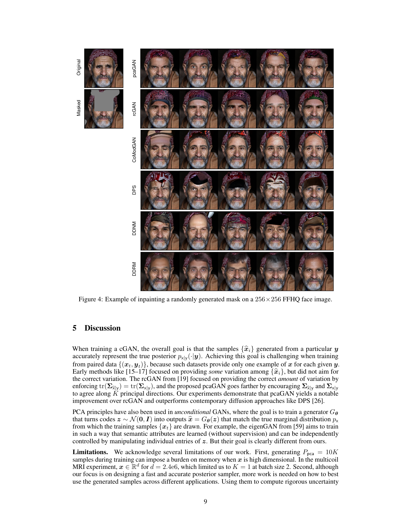
This figure shows the results of inpainting on a 256x256 FFHQ face image using different methods: Original, Masked, pcaGAN, rcGAN, CoModGAN, DPS, DDNM, and DDRM. Each method is represented by a row of images, showing multiple samples generated for a single masked image. This visualizes the diverse inpainting results produced by different approaches, allowing comparison of visual quality and diversity.

This figure shows the results of MRI recovery experiments at an acceleration factor of R=8. It compares the true image, the recovery generated by the proposed pcaGAN model, and several other methods (rcGAN, pscGAN, CGAN, and Langevin). The image shows the average reconstruction from 32 posterior samples (P=32) from each method. Also shown is a sample reconstruction from the posterior distribution of each method and the true image. The arrows highlight subtle differences in the reconstruction quality, demonstrating the effect of different methods on MRI recovery.
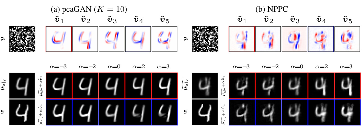
This figure compares pcaGAN and NPPC by visualizing the true image, noisy measurements, the conditional mean of the posterior distribution, the top 5 principal eigenvectors and two perturbed versions of the posterior mean for a specific MNIST digit. The perturbations are generated by adding multiples of each eigenvector to the mean, showcasing how the eigenvectors represent directions of variation in the posterior distribution.

This figure shows the results of MNIST denoising using both pcaGAN and NPPC. The top row shows the true image, the noisy measurement, and the top 5 principal eigenvectors generated by each method. The bottom row shows the reconstruction mean and two reconstructions obtained by adding and subtracting multiples of the principal eigenvectors to the mean. This helps illustrate how the principal components capture the uncertainty in the reconstruction.
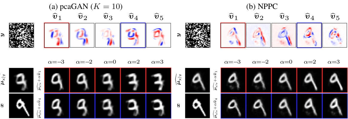
This figure shows the results of MNIST denoising using pcaGAN and NPPC. For each method, it displays the true image, the noisy measurement, the estimated posterior mean, the top 5 principal eigenvectors, and two images generated by adding multiples of the principal eigenvectors to the posterior mean. This illustrates how the principal components of the posterior distribution capture the uncertainty of the denoising process.
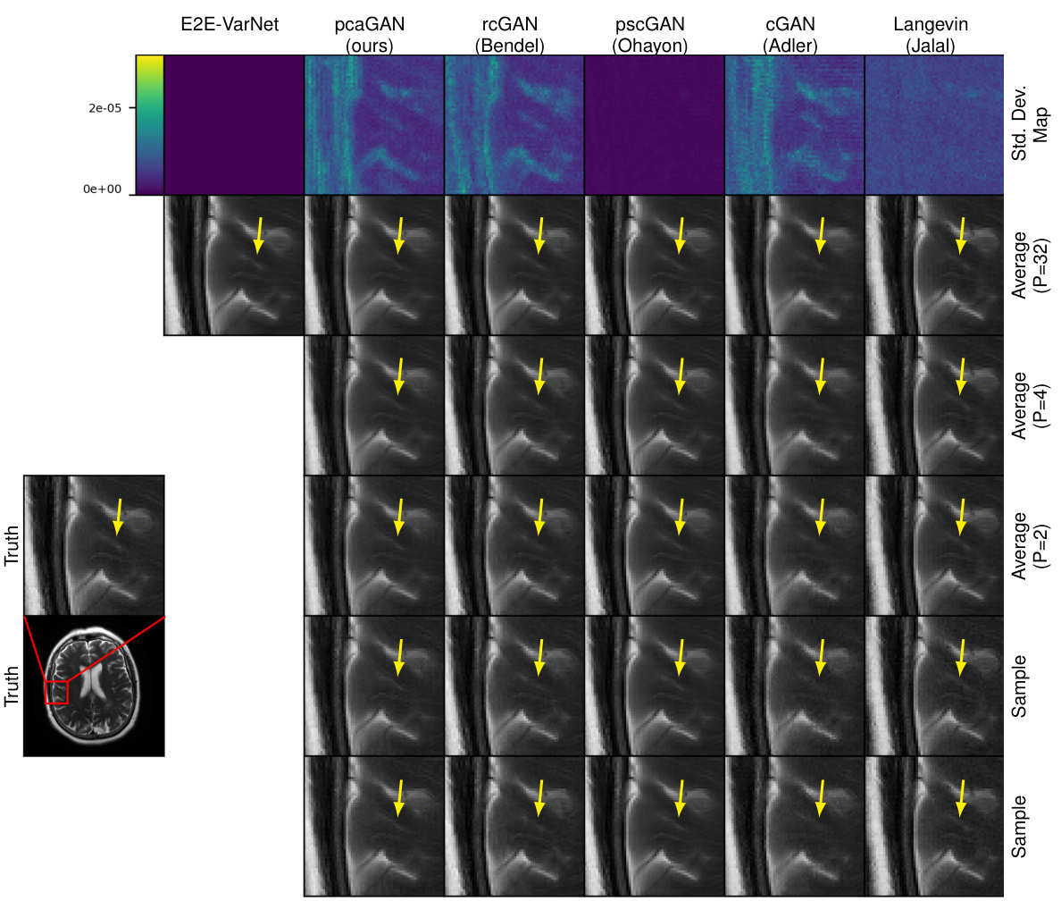
This figure shows the results of MRI reconstruction at an acceleration rate of R=4 using different methods. The top row displays the pixel-wise standard deviation for the posterior samples (P=32). The following rows show the average image generated from 2, 4, and 32 posterior samples. Finally, the last two rows show individual samples from the posterior distribution. The yellow arrows highlight variations between the different reconstructions.
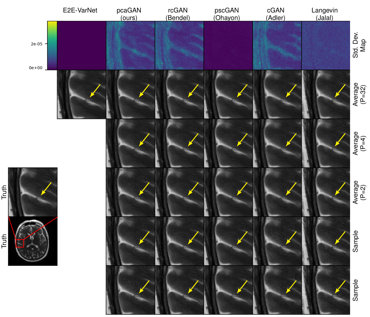
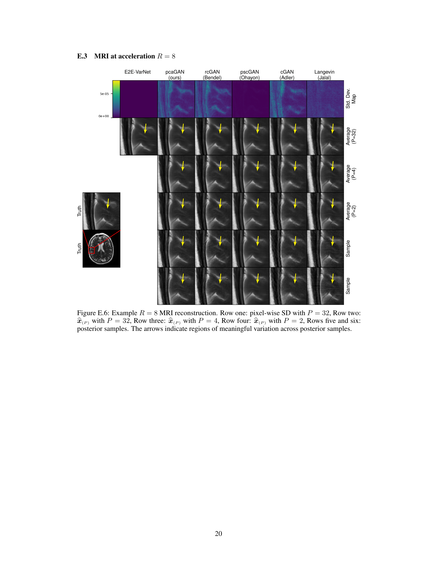
This figure shows the results of MRI reconstruction with acceleration factor R=8. The first row displays the pixel-wise standard deviation, and the following rows show the average reconstruction results and samples for different numbers of samples (P). The arrows highlight the meaningful variations in the reconstruction across the posterior samples.
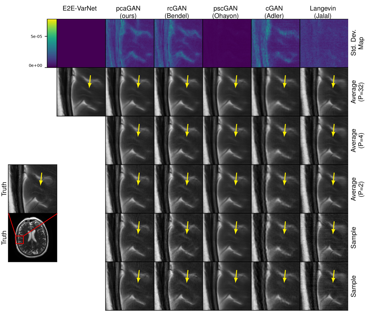
This figure shows the results of MRI reconstruction with acceleration factor R=4 using different methods. The first row displays the pixel-wise standard deviation (SD) when using 32 samples. The following rows show the average reconstruction results with 32, 4 and 2 samples. The last two rows show individual samples generated by each method, highlighting the variability in the posterior distribution of the reconstructions. The yellow arrows point out the image regions where the variability among samples is most apparent.
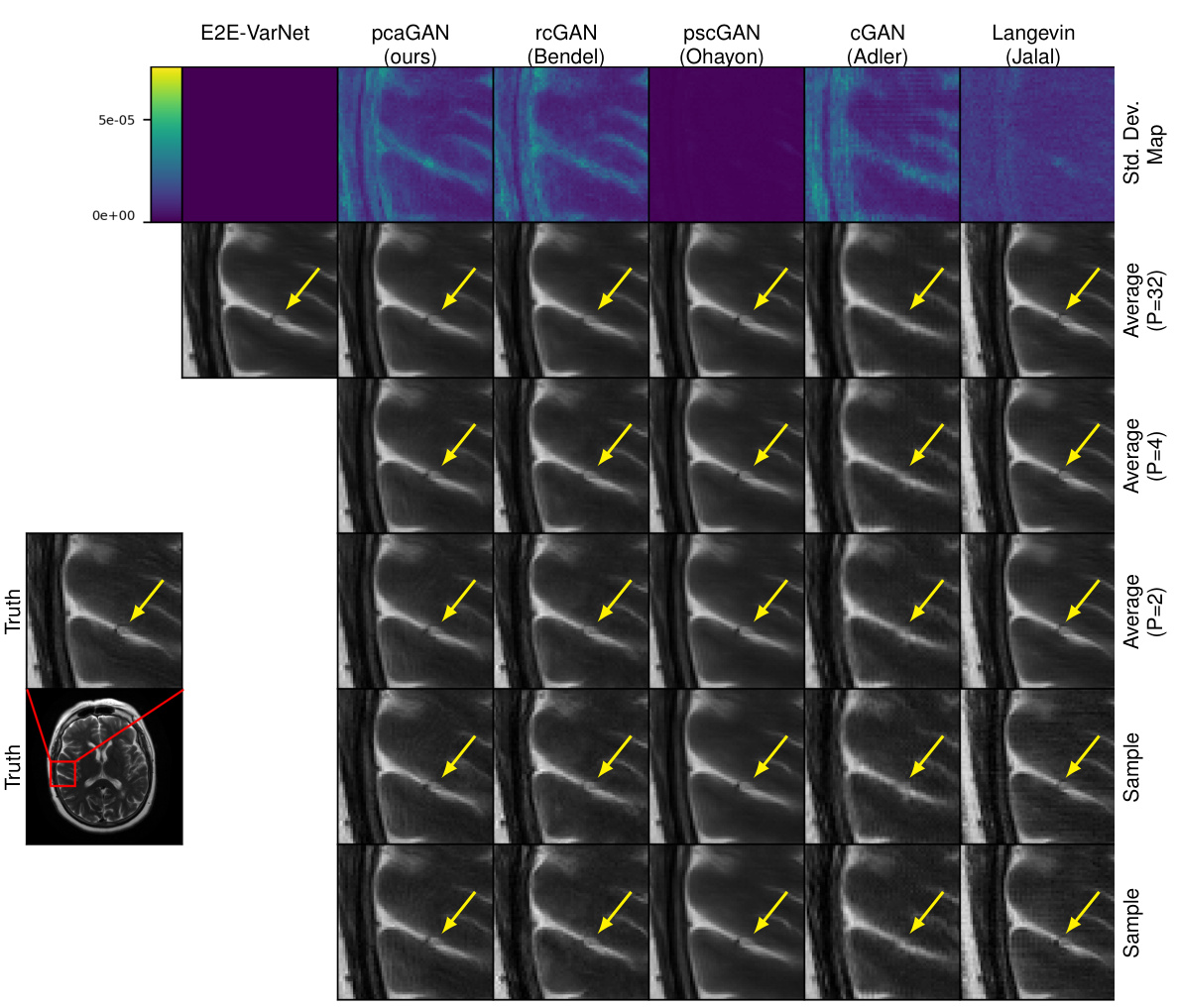
This figure shows the results of MRI reconstruction at acceleration rate R=8 using different methods. The top row displays the pixel-wise standard deviation (SD) of the posterior samples (P=32). The next three rows show the average reconstruction from 2, 4, and 32 posterior samples, respectively. Finally, the bottom two rows display individual samples from the posterior distribution. Yellow arrows highlight regions where the reconstruction varies meaningfully across posterior samples.
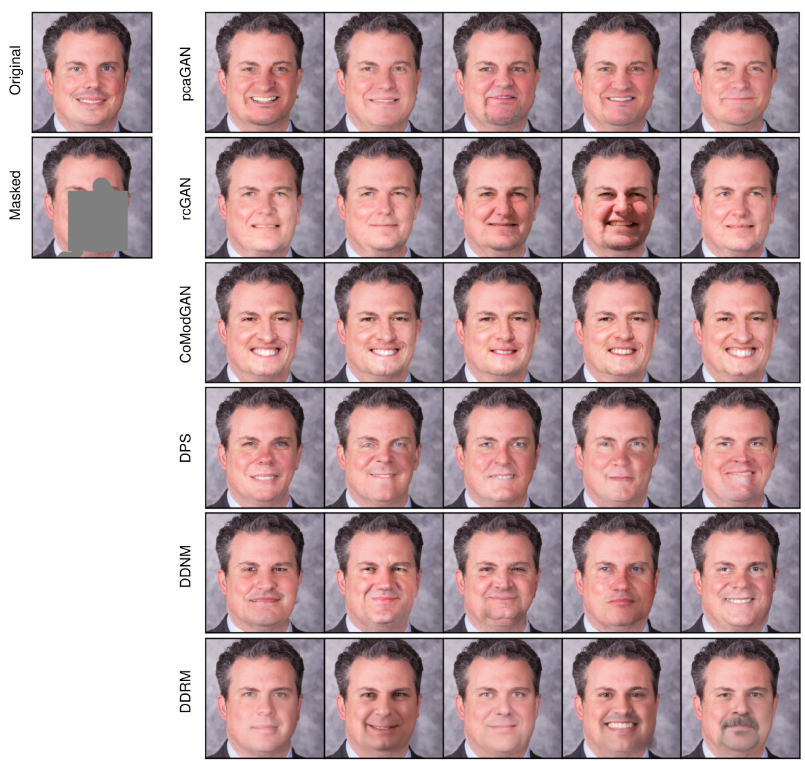
This figure shows the results of inpainting on a 256x256 FFHQ face image using different methods. The leftmost column shows the original image, followed by the masked image. Then, the subsequent columns present inpainting results from various models: DDRM, DDNM, DPS, CoModGAN, rcGAN, and pcaGAN. Each row shows the results obtained from the same model but with different samples from the posterior distribution. The figure visually demonstrates the quality and variety of inpainting achieved by each method.

This figure shows the results of inpainting a randomly generated mask on a 256x256 FFHQ face image using different methods. The original image is shown at the top left, followed by the masked image which has a significant portion of the face obscured. Below, the inpainting results for pcaGAN, rcGAN, CoModGAN, DPS, DDNM and DDRM are displayed, each method generating multiple samples to show variations in generated outputs. Visual comparison allows assessment of each method’s ability to realistically reconstruct the missing parts of the face, taking into account factors like texture, lighting, and overall facial features.
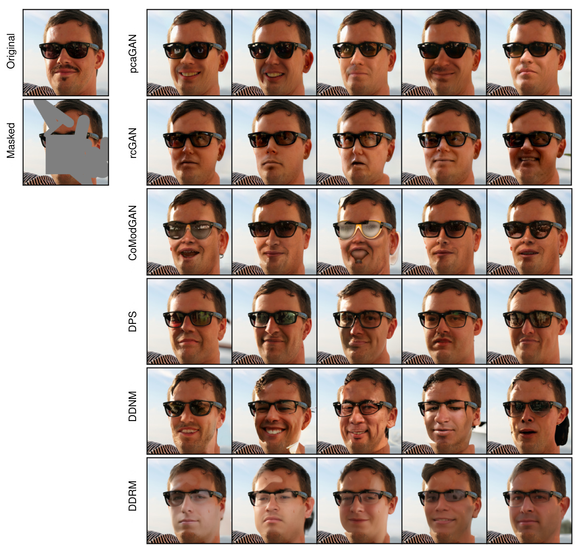
This figure shows the results of inpainting a randomly generated mask on several 256x256 FFHQ face images using different methods: pcaGAN, rcGAN, CoModGAN, DPS, DDNM, and DDRM. The ‘Original’ column shows the complete images. The ‘Masked’ column shows the same images with a random section masked out. The remaining columns show the inpainting results produced by each of the stated methods. The figure visually demonstrates the relative performance of each method in terms of the quality and realism of the inpainted regions.

This figure shows the results of inpainting on a 256x256 FFHQ face image using different methods. The ‘Original’ column shows the original image. The ‘Masked’ column shows the image with a randomly generated mask applied. The remaining columns display the inpainting results from several methods: pcaGAN (the authors’ method), rcGAN, CoModGAN, DPS, DDNM, and DDRM. The figure visually demonstrates the relative performance of each method in terms of the quality and realism of the inpainted region, as well as the diversity of results.
More on tables

This table presents the average results of different models for MRI reconstruction at acceleration rates R=4 and R=8. The metrics used for comparison include CFID (Conditional Fréchet Inception Distance) with three variations (CFID¹, CFID², CFID³ representing different numbers of test samples), FID (Fréchet Inception Distance), APSD (Average Perceptual Sample Distance), and the time taken for generating 4 samples. The models compared include E2E-VarNet, Langevin, cGAN (Adler & Oktem), pscGAN, rcGAN, and the proposed pcaGAN. The table showcases the performance of each model in terms of image reconstruction accuracy and computational efficiency.
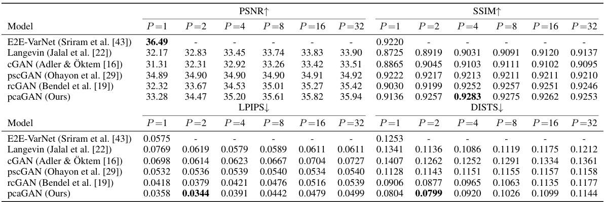
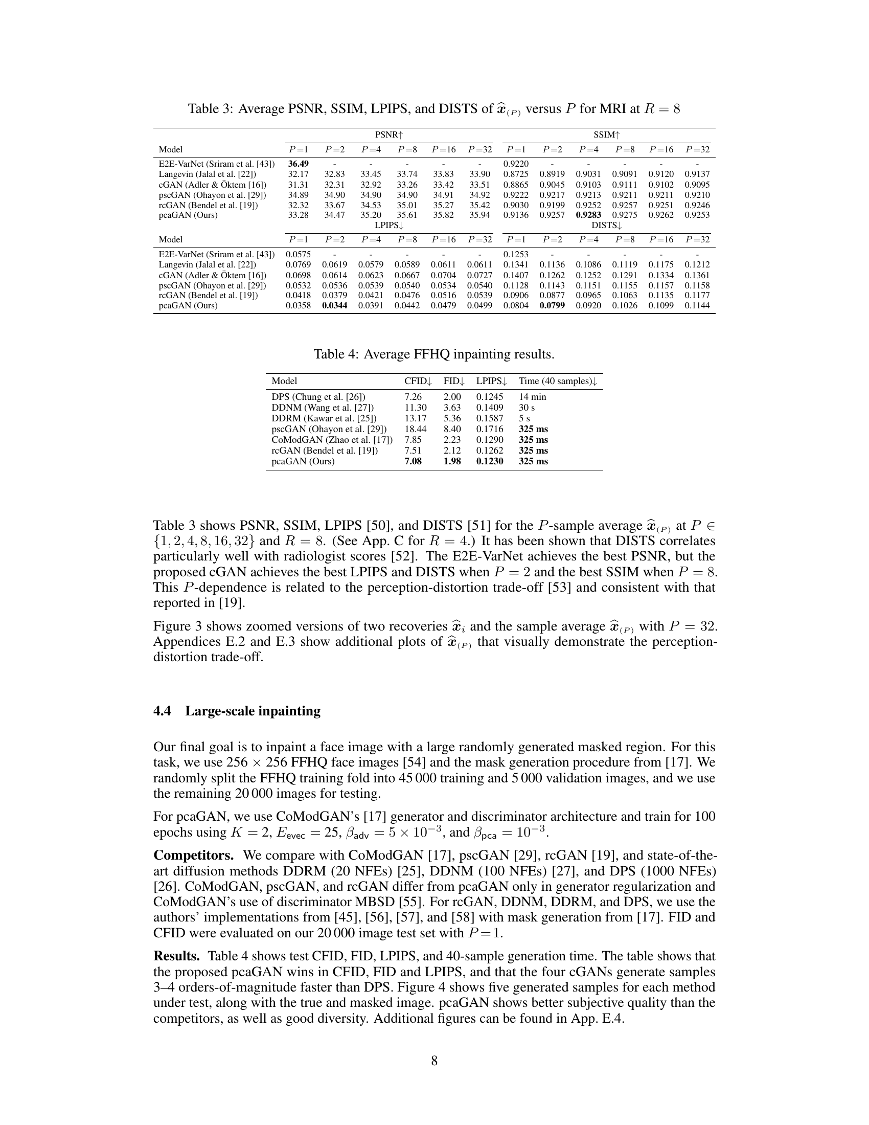
This table compares the performance of different models on MRI reconstruction task at acceleration factor R=8. It shows the PSNR, SSIM, LPIPS, and DISTS scores for different sample sizes (P). Higher PSNR and SSIM values indicate better reconstruction quality, while lower LPIPS and DISTS values indicate better perceptual similarity to the ground truth. The table helps to understand the trade-off between sample size and reconstruction quality.

This table presents the results of the FFHQ inpainting experiment. It compares different models (DPS, DDNM, DDRM, pscGAN, CoModGAN, rcGAN, and pcaGAN) in terms of their performance on inpainting tasks. The metrics used to evaluate performance include CFID, FID, and LPIPS. The table also shows the time taken to generate 40 samples for each method. The lower the CFID, FID, and LPIPS values, the better the performance. The table highlights that pcaGAN outperforms all other methods in terms of CFID, FID, and LPIPS and achieves comparable sample generation speed.

This table presents a comparison of different models on the MNIST denoising task. The models compared are NPPC, rcGAN, and two variants of the proposed pcaGAN (with K=5 and K=10). The metrics used for comparison are root mean squared error (rMSE), residual error magnitude (REM5), conditional Fréchet inception distance (CFID), and the average time taken to generate 128 samples. Lower values for rMSE, REM5, and CFID indicate better performance. The time metric indicates computational efficiency.

This table compares the performance of different models on MRI reconstruction with acceleration factor R=8. The metrics used are Peak Signal-to-Noise Ratio (PSNR), Structural Similarity Index (SSIM), Learned Perceptual Image Patch Similarity (LPIPS), and Distorted Image Similarity (DISTS). The results are shown for different numbers of samples (P) used to generate the average image. Higher PSNR and SSIM values indicate better image quality, while lower LPIPS and DISTS indicate better perceptual similarity to the ground truth.
Full paper#
