↗ OpenReview ↗ NeurIPS Homepage ↗ Chat
TL;DR#
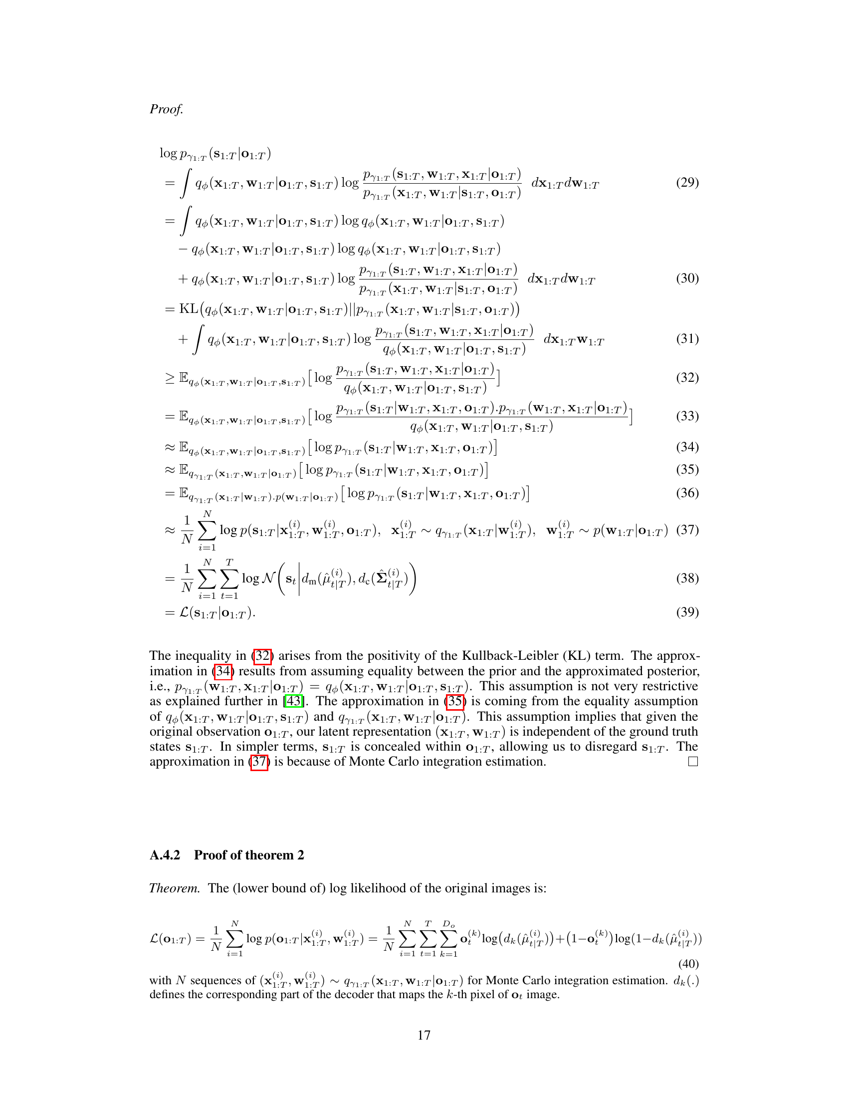
Many real-world applications, especially in fields like computer vision, deal with high-dimensional, noisy data exhibiting complex, nonlinear dynamics. Accurately estimating the underlying state (dynamics) from these observations is challenging due to computational cost and instability of existing methods. Traditional techniques like the extended Kalman filter (EKF) are often too slow or unstable for such complex scenarios.
This paper introduces GIN, a novel algorithm that solves these problems by efficiently approximating Bayesian inference for state-space models. GIN achieves this by disentangling the observations and their dynamics, using a compact recurrent neural network structure, and employing a specialized training method to handle exploding gradients. Experimental results demonstrate GIN’s superior performance on several benchmarks, showcasing its effectiveness in state estimation and missing data imputation.
Key Takeaways#
Why does it matter?#
This paper is important because it presents a novel and efficient algorithm for approximate Bayesian inference in state-space models with nonlinear dynamics. This is crucial for addressing challenges in high-dimensional, noisy data prevalent in many real-world applications like video processing. The proposed method, with its linear improvement in speed over traditional methods, opens avenues for advancing research in real-time state estimation and missing data imputation. The method’s focus on tackling the exploding gradient problem is also highly relevant to deep learning research.
Visual Insights#

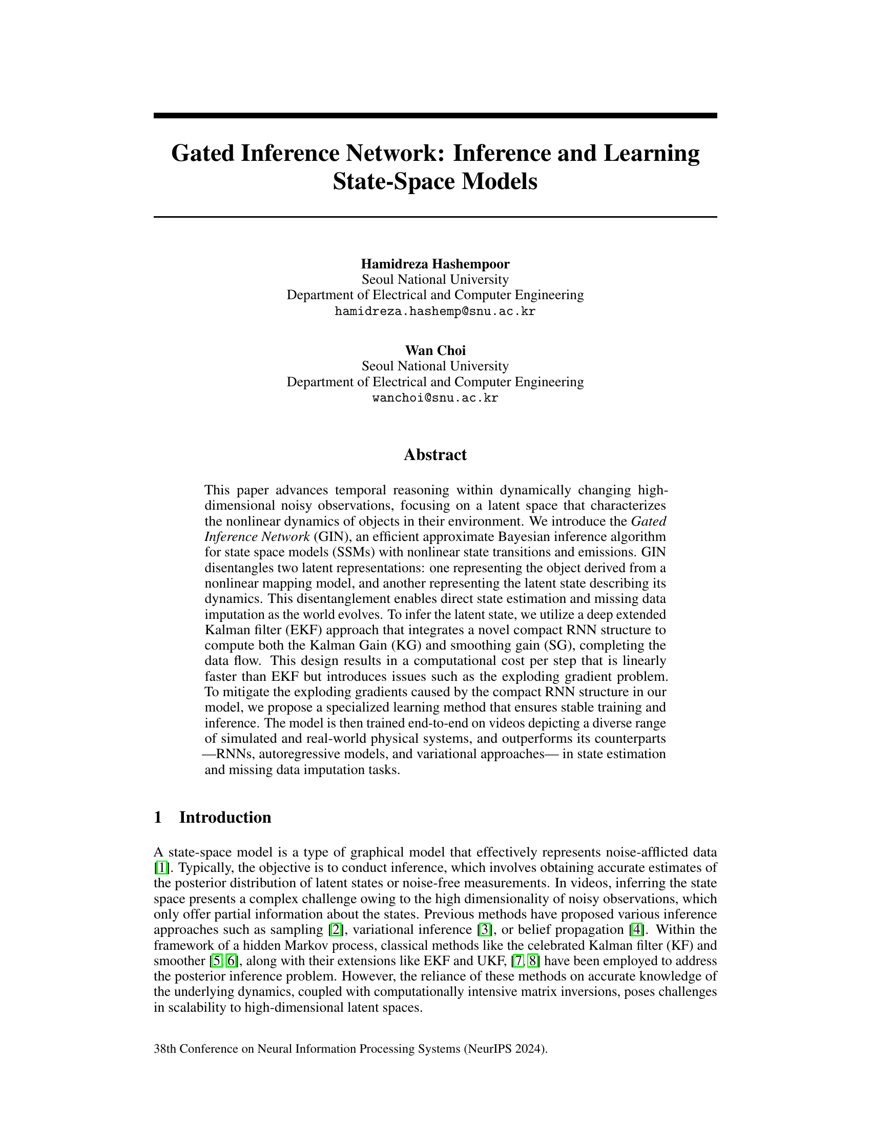
This figure shows several frames from videos generated by the Gated Inference Network (GIN) model. Each frame is a single image, representing one time step in a sequence. The color intensity within each image represents the progression of time within the sequence, with darker shades indicating earlier time steps. The videos depict a ball moving within irregular polygon environments. The figure highlights the model’s ability to generate plausible and temporally consistent sequences of video frames.

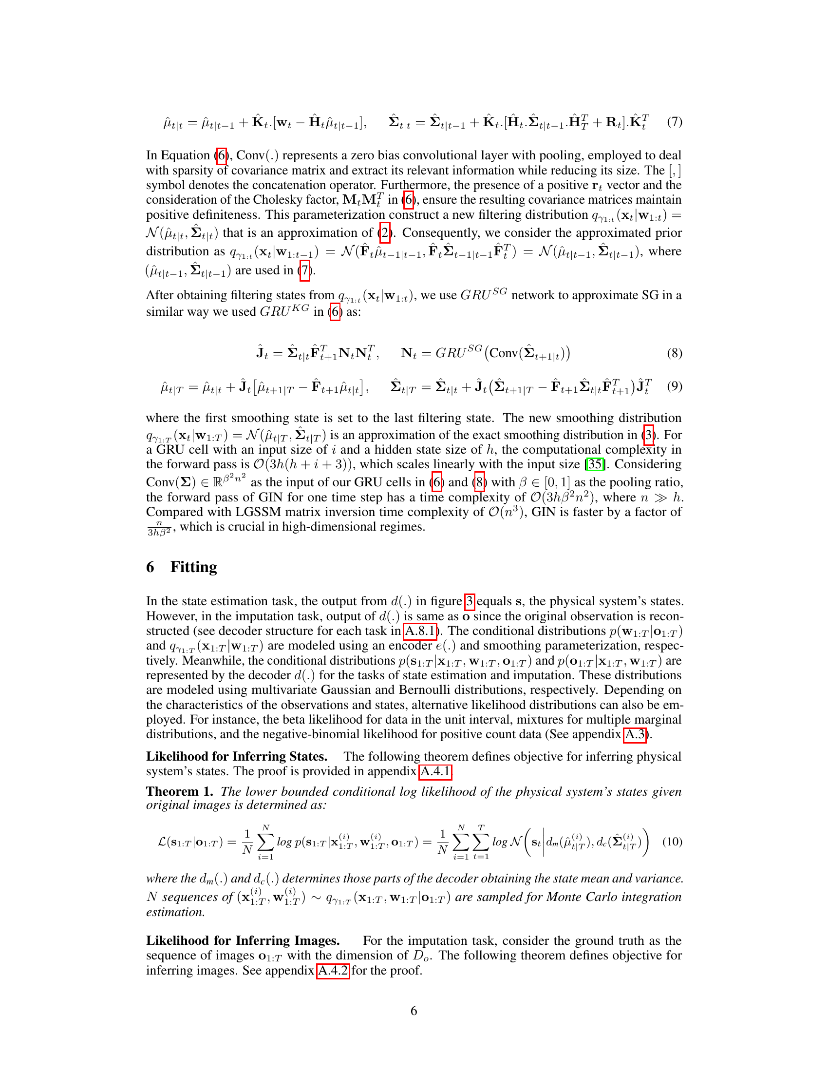
This table presents the results of state estimation experiments conducted on double pendulum, single pendulum, and irregular polygon scenarios. For each model, it shows the Squared Error (SE) in estimating the state variables (positions of joints/ball) and the log-likelihood achieved. The table compares the performance of various models, including the proposed GIN and several baselines (VAE, RNNs, etc.). The SE values reflect the accuracy of state estimation, with lower values indicating higher accuracy. The log-likelihood shows how well the models fit the observed data, with higher values suggesting a better fit. The table helps to illustrate the performance of the GIN in comparison to other models.
In-depth insights#
Gated Inference#
Gated inference, in the context of a research paper likely dealing with state-space models or sequential data, suggests a mechanism for controlling the flow of information during inference. It likely involves using gates, similar to those in recurrent neural networks (RNNs), to selectively allow or block the passage of information based on context or learned criteria. This could lead to improved efficiency by focusing computational resources on relevant parts of the data. A gated mechanism could also improve robustness to noise or irrelevant information. The gating could be learned from the data itself, making the inference process more adaptive and flexible. The overall approach is likely designed to approximate Bayesian inference, which is often intractable for high-dimensional data. Thus, the use of gating implies a clever method of approximation. The key benefit of the gated architecture might be a balance between the complexity of the inference and computational efficiency. By selectively attending to information, the model can avoid processing irrelevant or noisy data, resulting in faster inference and potentially, better accuracy.
Nonlinear SSMs#
Nonlinear state-space models (SSMs) significantly extend the capabilities of linear SSMs by accurately representing real-world systems that exhibit nonlinearities in their state transitions or emissions. Nonlinearity is crucial for capturing the complex dynamics of many physical and biological processes, which are often not well-approximated by linear functions. Approaches for handling nonlinear SSMs include extended Kalman filters (EKFs) and unscented Kalman filters (UKFs) which linearize the system or use a sampling approach to approximate the posterior distribution. However, these methods often struggle in high-dimensional spaces or with severe nonlinearities. Deep learning methods, such as recurrent neural networks, provide a promising alternative by learning complex nonlinear mappings from data, and they can be used to approximate the posterior distribution or directly model the state transitions and emissions. A major challenge in working with nonlinear SSMs is the increased computational cost and potential for numerical instability. Effective inference techniques, such as variational inference or particle filtering, are often necessary to handle these challenges.
GRU-based KG/SG#
The use of GRUs to compute the Kalman Gain (KG) and smoothing gain (SG) is a key innovation in this paper. Instead of the computationally expensive matrix inversions typically used in Extended Kalman Filters (EKFs), the authors leverage the recurrent nature of GRUs to efficiently approximate KG and SG. This approach significantly reduces the computational complexity, making the algorithm linearly faster than traditional EKFs. While computationally efficient, using GRUs introduces challenges, specifically the potential for exploding gradients. The paper acknowledges this and proposes a specialized learning method to mitigate this issue and ensure stable training and inference. The effectiveness of this novel GRU-based KG/SG approach is demonstrated through experiments on various simulated and real-world datasets, showing improved performance over traditional methods. This efficient and robust method allows for scalable temporal reasoning in high-dimensional spaces.
Gradient Mitigation#
In training deep neural networks, particularly those with recurrent structures like the GRUs used in this paper’s Gated Inference Network (GIN), exploding gradients pose a significant challenge. Gradient mitigation techniques are crucial for ensuring stable training and preventing the network from diverging. The core problem is the multiplicative nature of gradients in RNNs, where errors accumulate over time, potentially leading to extremely large values that disrupt the learning process. The paper addresses this by proposing a specialized learning method. This method likely involves either constraining the magnitude of gradients (gradient clipping), regularizing the network’s parameters (weight decay or other forms of regularization), or employing a more sophisticated optimization algorithm designed to handle unstable gradients (e.g., adaptive optimization methods like Adam). Understanding the specific approach used in the paper would require deeper analysis of the provided PDF. Regardless of the precise method, the goal is to maintain the network’s stability during training, ultimately leading to improved performance in the state estimation and missing data imputation tasks.
Future Directions#
Future research could explore several promising avenues. Extending the GIN to handle more complex scenarios, such as those involving occlusions or changes in lighting conditions, is crucial for real-world applicability. Improving the efficiency of the RNN structure within GIN is essential to handle longer sequences and higher-dimensional data. The current RNN structure, while computationally efficient, could still be improved to handle more complex dynamics. Investigating alternative training methodologies, potentially incorporating techniques like reinforcement learning, could enhance GIN’s robustness and efficiency. Exploring the potential of combining GIN with other deep learning methods, such as those used for object detection or tracking, would be useful in creating comprehensive perception systems. Finally, a thorough investigation into the theoretical properties of GIN, including its convergence and stability guarantees, would strengthen its foundation and guide further advancements.
More visual insights#
More on figures
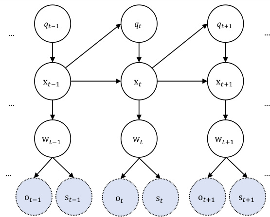
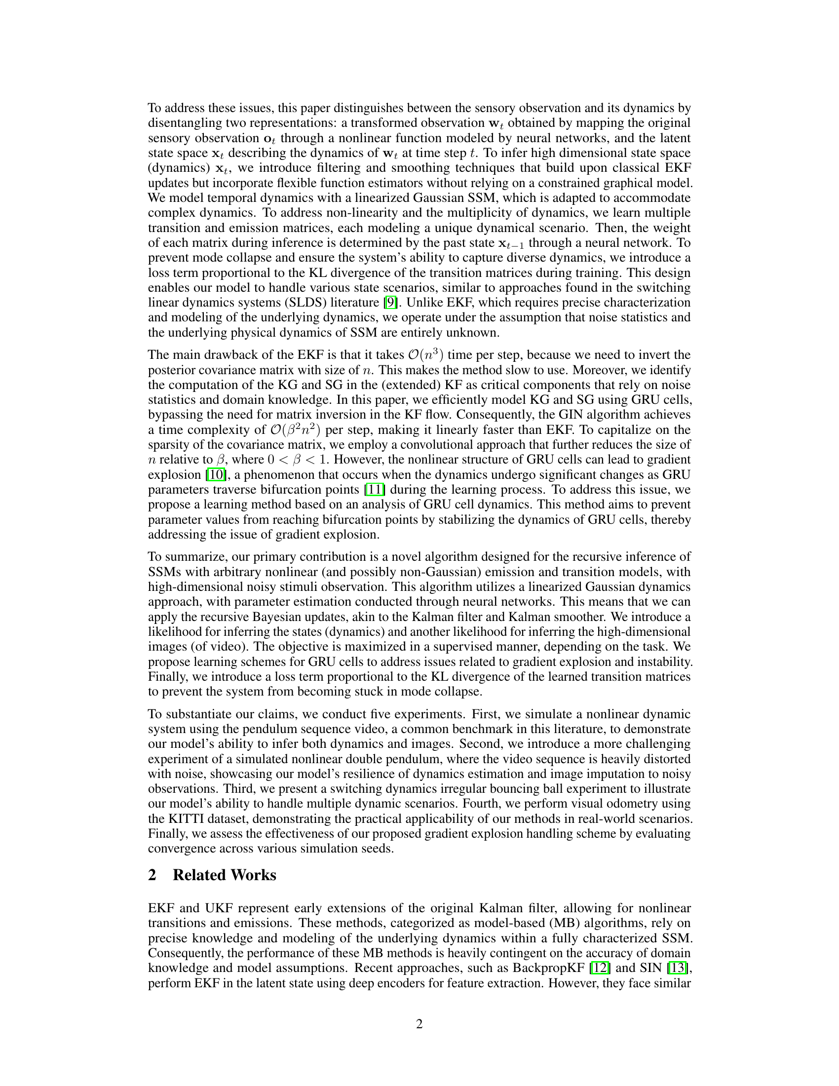
This figure shows a graphical model representing the relationships between variables in the Gated Inference Network (GIN). The nodes represent variables, such as latent states (x), transferred observations (w), original observations (o), and task-dependent outputs (s). The arrows indicate the probabilistic dependencies between the variables. Dashed nodes represent task-dependent outputs, meaning that their presence and values depend on the specific task being performed (either state estimation or image imputation). The model demonstrates the flow of information and the dependencies between sensory observations, latent states, and the final outputs.

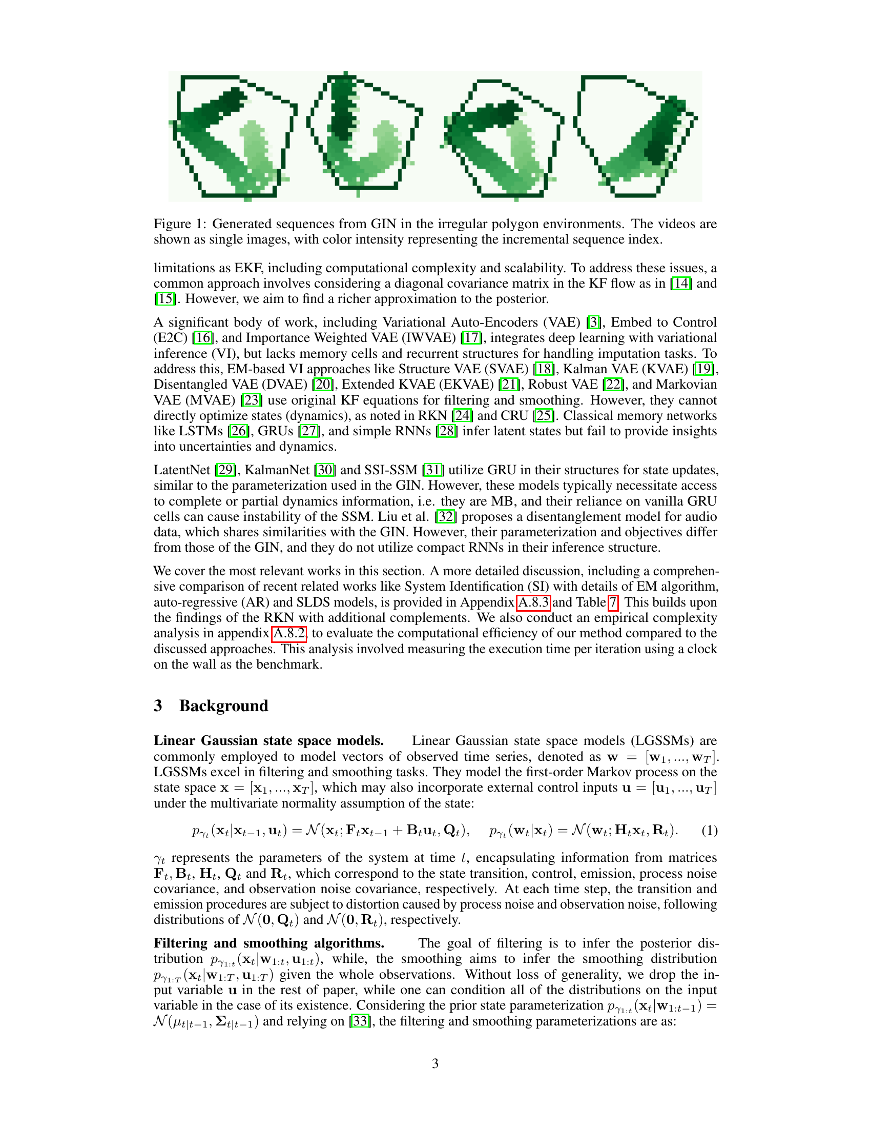
This figure illustrates the Gated Inference Network (GIN) as a Hammerstein-Wiener (HW) model. The GIN consists of three main components: an encoder (e(.)), a transition block, and a decoder (d(.)). The encoder maps the original high-dimensional sensory observations (o1:T) to a lower-dimensional representation (w1:T). The transition block models the temporal dynamics of the system, updating the latent states (x1:T) based on the transformed observations. Finally, the decoder maps the latent states and transformed observations to the task-specific output, which can either be the original observations (denoised and imputed) or the physical system’s states (s1:T). The flexibility of the GIN comes from its ability to handle high-dimensional observations through the appropriate selection of the encoder and decoder structures, e(.) and d(.).

This figure details the transition block’s operation within the Gated Inference Network (GIN). It shows how, at each time step, the posterior probability of the previous state (xt−1|W1:t−1) is used by the Dynamic Network to estimate parameters, these estimates along with the current observation (wt) are used to obtain a filtered state estimate (xt|W1:t), and finally, combining the filtered estimate with a smoothed estimate of the next state (xt+1|W1:T) yields a smoothed estimate for the current state (xt|W1:T). This process involves both filtering and smoothing steps to achieve accurate state estimation within a dynamic system.
This figure shows a series of images generated by the Gated Inference Network (GIN) model while simulating a ball bouncing inside an irregular polygon. Each image represents a single frame from a video sequence, with the color intensity indicating the time progression within the sequence. The irregular polygon environment introduces complex dynamics due to the changing boundary conditions as the ball collides with the walls of the polygon at various angles and locations. The figure showcases the GIN’s ability to generate realistic and coherent video sequences in a challenging dynamic environment, where the object’s motion is not predictable.

This figure shows a series of images generated by the Gated Inference Network (GIN) model while simulating a ball bouncing inside an irregular polygon. Each image represents a single frame from a video sequence, and the color intensity corresponds to the frame’s position within the sequence. It demonstrates the model’s ability to handle and represent dynamic situations. The irregular polygon shape indicates the model’s capacity to manage varying scenarios.
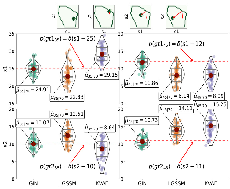
The figure displays the state estimation results for a bouncing ball in a hexagon-shaped environment at the 35th and 45th time steps. The top row shows the ground truth ball positions. The bottom rows showcase the estimated positions from the GIN, LGSSM, and KVAE models. The results highlight how the GIN more accurately predicts the ball’s position compared to the other models, especially in irregular polygon environments.

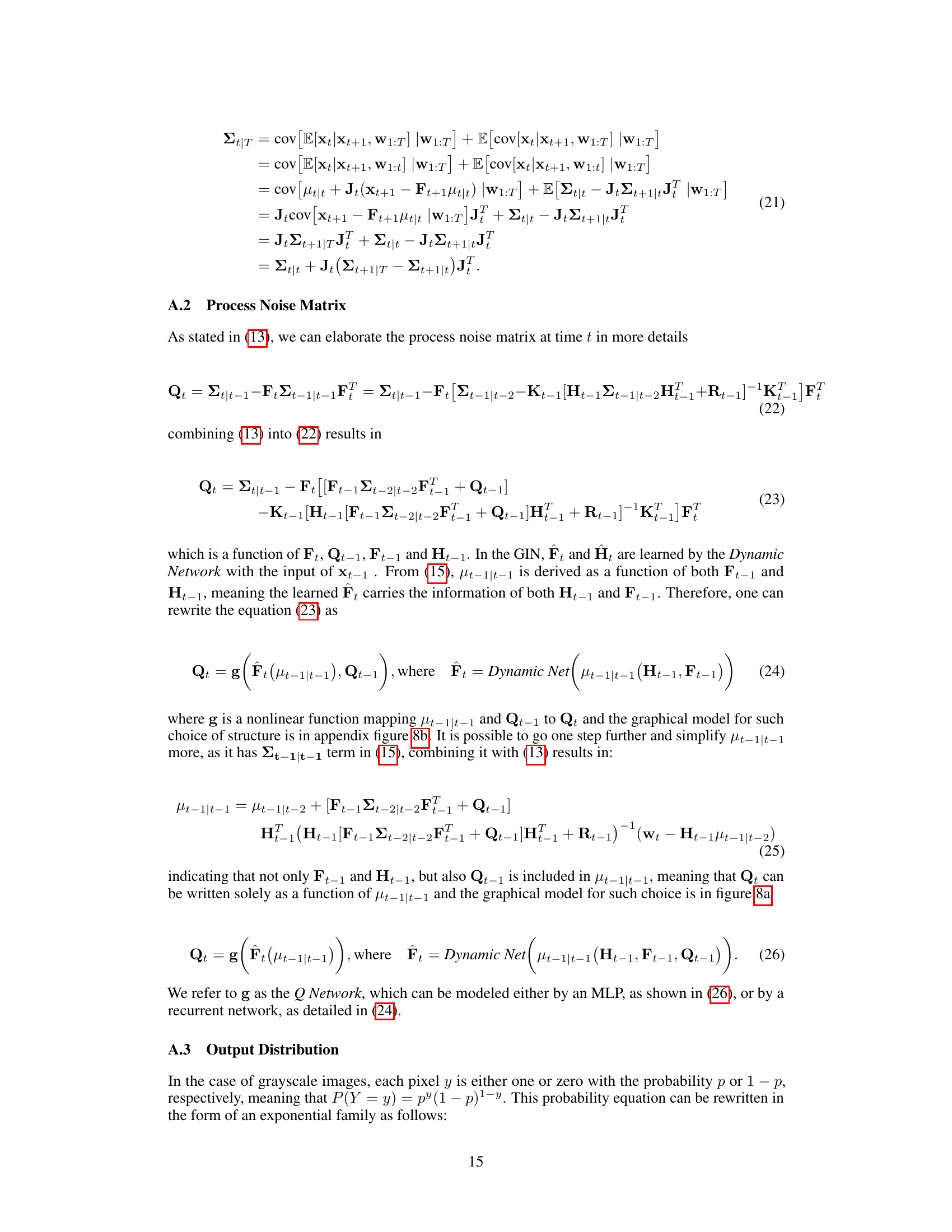
The figure shows two graphical models representing different parameterizations for the process noise in the Gated Inference Network (GIN). Model (a) depicts a simpler model where the process noise, Qt, is parameterized as a function of the previous state’s posterior mean (µt−1|t−1), the previous process noise (Qt−1), and the learned transition and emission matrices (Ft and Ht). The model in (b) is more complex with an explicit recurrent structure where Qt depends on the previous process noise, Qt−1, through a recurrent connection.
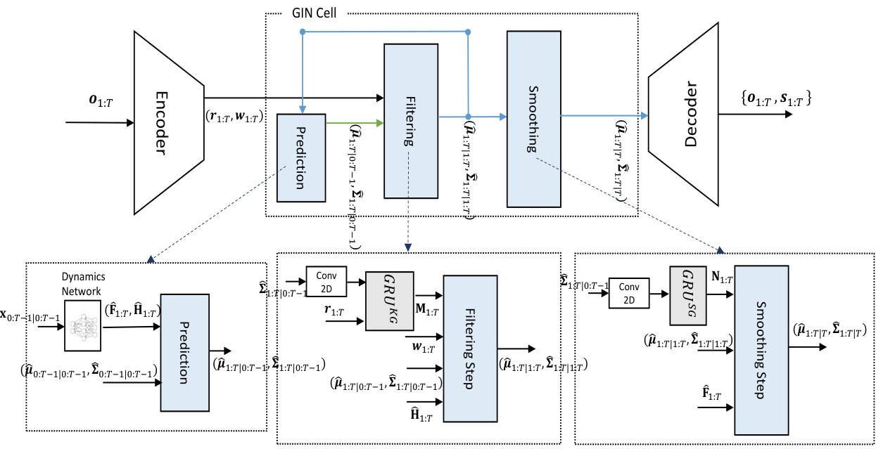
This figure illustrates the Gated Inference Network (GIN) architecture as a Hammerstein-Wiener (HW) model. The GIN disentangles observations into two representations: a transformed observation (wt) obtained by a nonlinear mapping (e(.)) from the original observation (ot), and a latent state (xt) that describes the dynamics of wt. The transition block, a core component of the GIN, simulates the relationship between wt and xt to infer the high-dimensional state space.
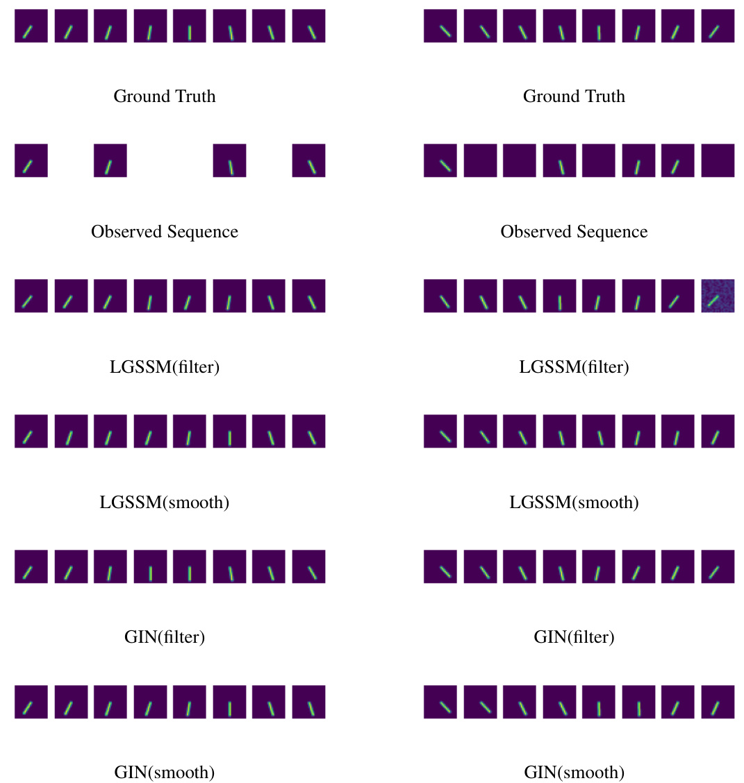
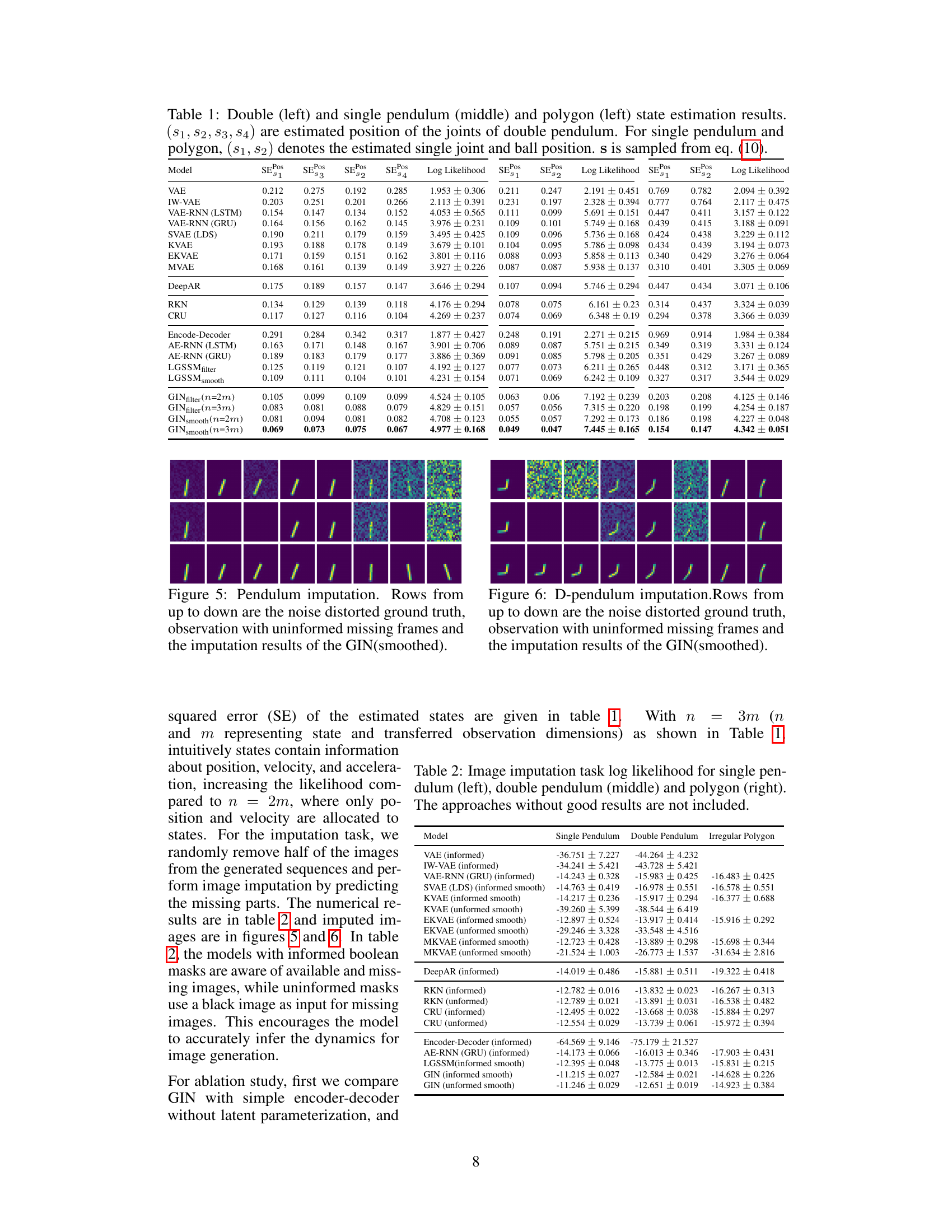
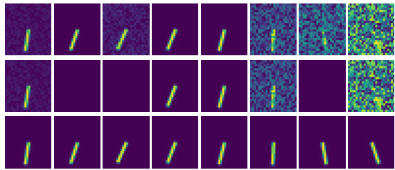
This figure shows the results of image imputation for a single pendulum experiment. The left column shows the results when the model is given information about which frames are missing (informed). The right column displays the results when the model is not given this information (uninformed). The top row is the ground truth sequence of images. The second row presents the observed sequence with missing frames (represented by black images). The following rows show the reconstruction using LGSSM (filtering and smoothing) and GIN (filtering and smoothing), respectively. The results illustrate the model’s ability to handle missing data and the potential benefits of using informed masks, given the superior performance of the informed approach.

This figure shows a sequence of images generated by the Gated Inference Network (GIN) model. Each image represents a frame from a video sequence, where the color intensity indicates the time progression. The model simulates a bouncing ball within irregularly shaped polygons, demonstrating the GIN’s ability to capture complex dynamics.

This figure shows the results of image imputation experiments for a single pendulum. The top row displays the ground truth images. The middle row shows the observed sequence, which has missing frames. The bottom rows show the reconstruction of the missing frames using LGSSM (filter), LGSSM (smooth), GIN (filter), and GIN (smooth). The left column represents experiments using an informed mask, where the model knows which frames are missing, while the right column depicts uninformed masks, where the model is given just black images for the missing frames.

This figure shows a series of images generated by the Gated Inference Network (GIN) model. Each image represents a single frame from a video sequence of a ball bouncing in an irregularly shaped polygon. The color intensity in each image indicates the time progression of the video sequence, allowing one to visually track the movement of the ball over time.

This figure compares the performance of three different models (GIN, LGSSM, and KVAE) in estimating the state of a single pendulum at a specific time step (100th). The violin plots show the distributions of samples generated from the smoothened state distribution for each model. The red dashed line indicates the ground truth state, which is compared to the estimated states to assess each model’s accuracy. The plot provides a visual comparison of the accuracy and uncertainty of each model’s estimations.

This figure shows the inference results for the single pendulum’s first joint position (s1) at the 100th time step. It compares the generated samples from the smoothed distribution obtained using three different methods: GIN, LGSSM, and KVAE. The dashed red line indicates the ground truth state’s distribution, centered at 0.7. The plot provides a visual comparison of the three models’ performance in estimating this specific position, highlighting differences in accuracy and uncertainty.

This figure compares the performance of three different models (GIN, LGSSM, and KVAE) in estimating the joint distribution of the single pendulum’s position at time step 100. Each subplot displays a 2D density plot showing the probability distribution of the pendulum’s position in the s1 and s2 dimensions. The black point represents the ground truth values for s1 and s2 at time step 100. The spread and shape of the distributions illustrate the accuracy and uncertainty of each model’s estimate.

This figure compares the performance of three different models (GIN, LGSSM, and KVAE) in estimating the state of a double pendulum at a specific time step (100th). It shows the distributions of generated samples from the models’ smoothened distribution for the first joint’s position (s1), which is compared against the ground truth. The red dashed line indicates the ground truth state.
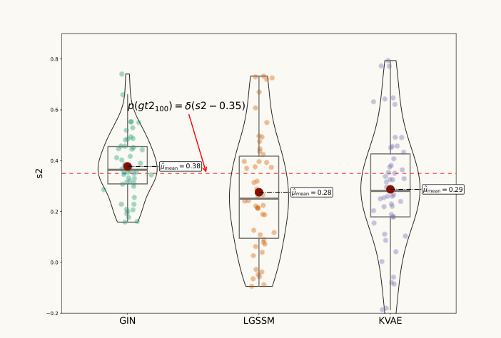
This figure shows the inference results for the double pendulum’s second joint position (s2) at the 100th time step. It presents generated samples from the smoothened distribution, comparing the performance of the Gated Inference Network (GIN), the Linear Gaussian State Space Model (LGSSM), and the Kalman Variational Autoencoder (KVAE). The ground truth state distribution is also indicated by a dashed red line.

This figure shows the comparison of the performance of GIN, LGSSM, and KVAE in estimating the joint distribution of the double pendulum’s second joint position at time step 100. The plots display the estimated distributions as density maps, allowing for a visual comparison of the accuracy and uncertainty of each model’s predictions. The ground truth is shown as a black point for reference.
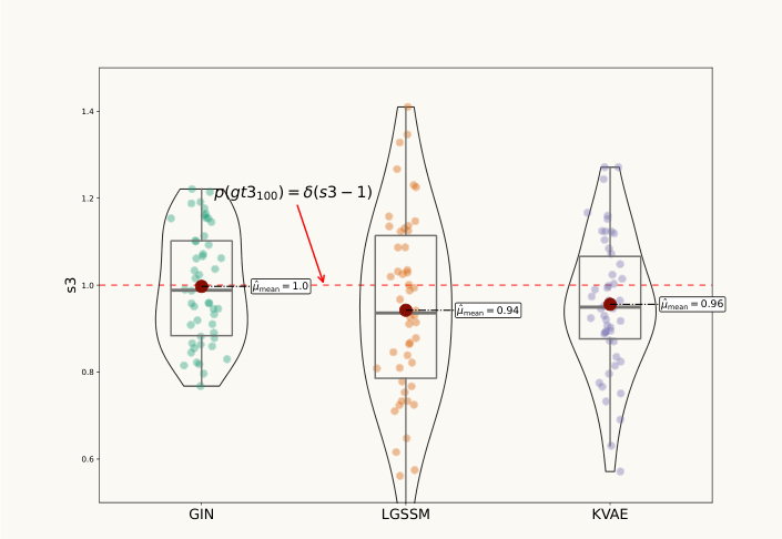
The figure shows the inference results for the single pendulum’s s1 position at the 100th time step. It presents violin plots comparing the generated samples from the smoothened distribution obtained using three different methods: GIN, LGSSM, and KVAE. The plots show the distribution of the samples, highlighting the difference in uncertainty and accuracy of each method. A dashed red line indicates the ground truth state.

This figure compares the state estimations of the GIN, LGSSM, and KVAE models for the single pendulum’s s1 position at the 100th time step. The GIN’s estimates show a tighter distribution around the ground truth (red dashed line), indicating better accuracy and lower uncertainty compared to the other two methods.

This figure compares the performance of three different models (GIN, LGSSM, and KVAE) in estimating the joint distribution of the double pendulum’s second joint position (s3, s4) at the 100th time step. The generated samples from the smoothened distributions are shown as contour plots, with the ground truth marked by a black point. The plots visualize the uncertainty and accuracy of each model’s prediction, providing a visual comparison of their performance in state estimation.

This figure shows the results of visual odometry experiments using GIN, LGSSM, and KVAE. Specifically, it displays the generated samples from the smoothened distribution of the visual odometry’s s1 and s2 positions at the 100th time step. The red dashed lines represent the ground truth state distributions.

This figure shows the visual odometry results at the 100th time step. It compares the performance of the GIN, LGSSM, and KVAE models in estimating the s1 and s2 positions. The ground truth is represented by a dashed red line, indicating a distribution centered around specific values. The violin plots visually represent the distribution of samples generated from the smoothened distribution obtained by each model, giving an idea of the uncertainty associated with each model’s estimation. The GIN shows better performance in terms of both accuracy and lower uncertainty.
More on tables
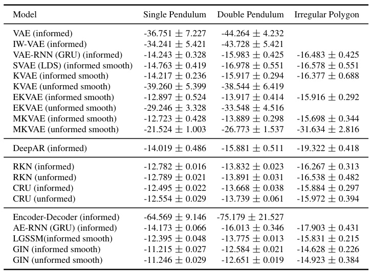
This table presents the log-likelihood results for image imputation experiments across three different scenarios: single pendulum, double pendulum, and irregular polygon. The results are separated into informed and uninformed cases, indicating whether the model knew which image frames were missing or not. The table compares the performance of various models, such as VAE, IWVAE, VAE-RNNs, SVAE, KVAE, EKVAE, MVAE, DeepAR, RKN, CRU, an encoder-decoder, AE-RNNs, and LGSSM, against the GIN (both informed and uninformed). The lower log-likelihood values indicate better performance in image imputation.

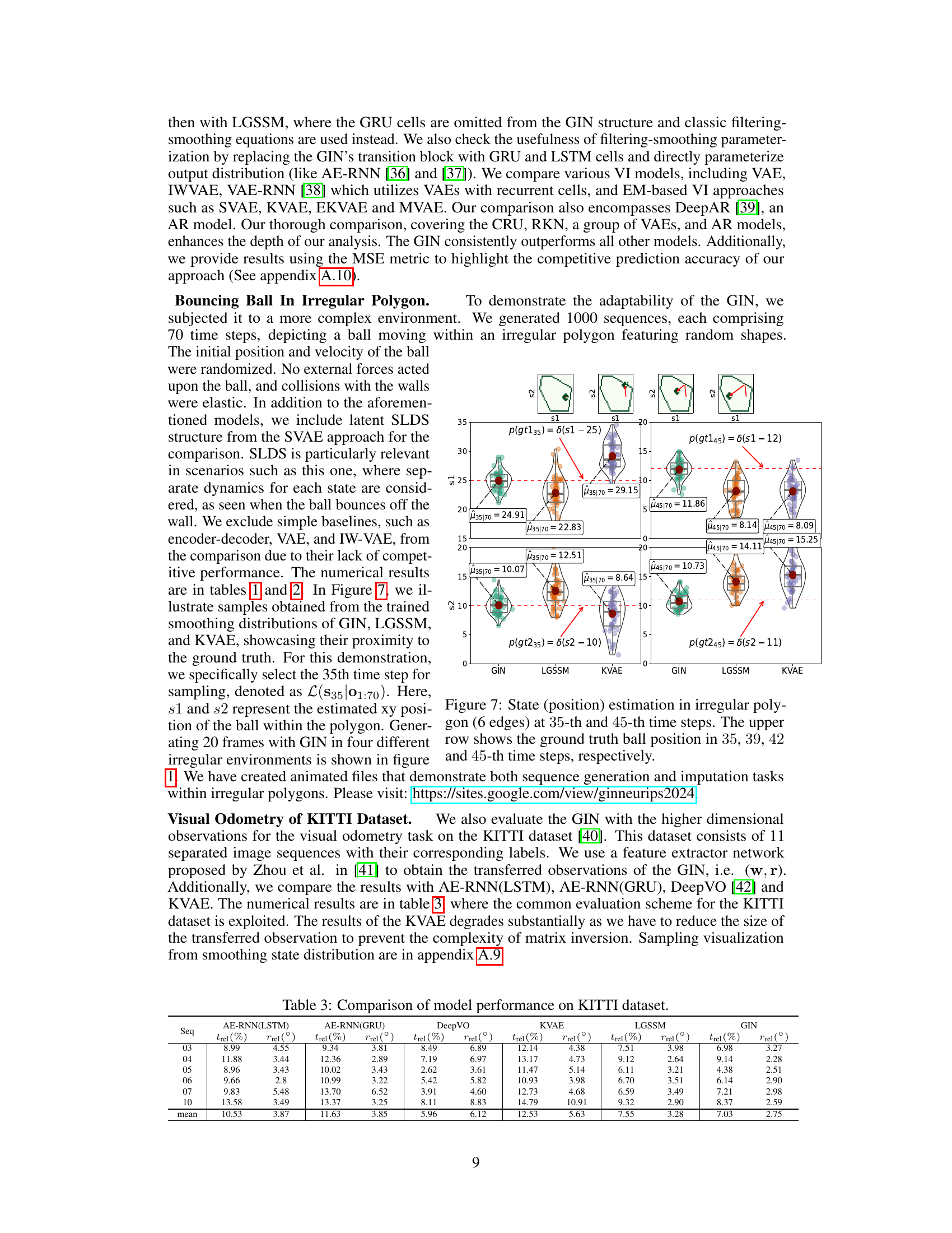
This table compares the performance of different models (AE-RNN(LSTM), AE-RNN(GRU), DeepVO, KVAE, LGSSM, and GIN) on the KITTI visual odometry dataset. The metrics used are translation error (trel) and rotation error (rrel) in percentage and degrees respectively. The results show the average performance across different sequences in the dataset.

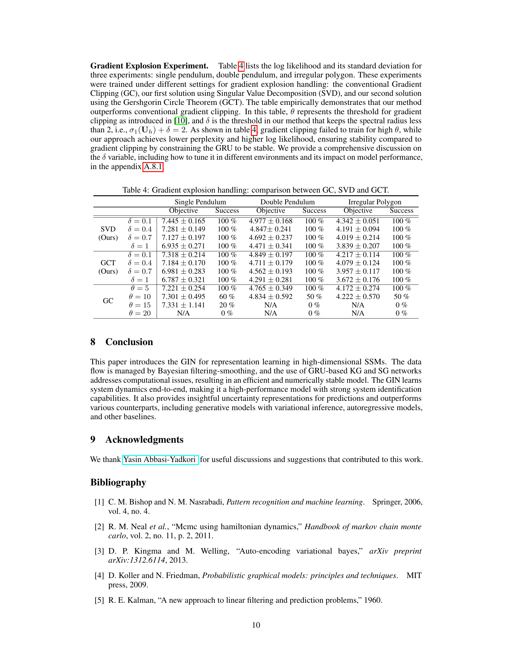
This table presents the results of experiments conducted to evaluate the effectiveness of different methods for handling gradient explosion during the training process. Three methods are compared: conventional Gradient Clipping (GC), the first proposed solution using Singular Value Decomposition (SVD), and the second proposed solution using the Gershgorin Circle Theorem (GCT). The table shows the objective function values and success rates for each method across three different experiments: single pendulum, double pendulum, and irregular polygon. The success rate indicates whether the training process successfully converged for a given hyperparameter setting. The different values of δ and θ represent the hyperparameters used in the different gradient explosion handling methods.

This table compares various algorithms (LSTM, GRU, VAE, IW-VAE, VAE-RNN, SVAE, KVAE, EKVAE, MVAE, DeepAR, RKN, CRU, Encode-Decoder, AE-RNN, LGSSM, and GIN) in terms of their computational efficiency and the number of parameters used. The comparison is done across four tasks: single pendulum, double pendulum, bouncing ball, and visual odometry. The table showcases the GIN’s efficiency compared to other methods in terms of both parameter count and running time.
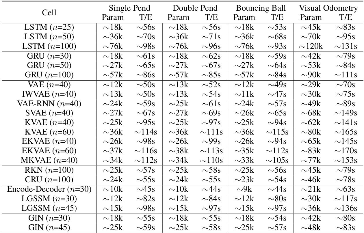
This table compares various algorithms based on their empirical running times and the number of parameters used for different experiments (single pendulum, double pendulum, bouncing ball, visual odometry). The comparison covers various model types, including LSTMs, GRUs, VAEs, and the proposed GIN, highlighting the efficiency of the GIN in terms of both computational cost and parameter count. The table provides insights into the trade-off between model complexity and performance for different tasks.

This table compares the performance of various models on the KITTI dataset for visual odometry. It shows the translation error (trel) and rotation error (rrel) for different image sequences, providing a quantitative comparison of the GIN against other state-of-the-art approaches. The table highlights the GIN’s strengths in handling high-dimensional data, learning dynamics, and accurate state estimation.

This table presents the Mean Squared Error (MSE) results for a single pendulum experiment. Different model architectures (LSTM and GRU with varying numbers of units and observation dimensions (m)) are compared to assess their performance in state estimation. Lower MSE values indicate better performance.
This table presents a comparison of the state estimation results for three different scenarios: double pendulum, single pendulum, and a ball in a polygon. Several models are evaluated, and their performance is measured using the Squared Error (SE) for the estimated positions of the pendulum joints and the ball. The table shows the mean SE, along with log-likelihood values indicating how well each model fits the data. The results highlight the performance of the GIN model in comparison to existing methods.

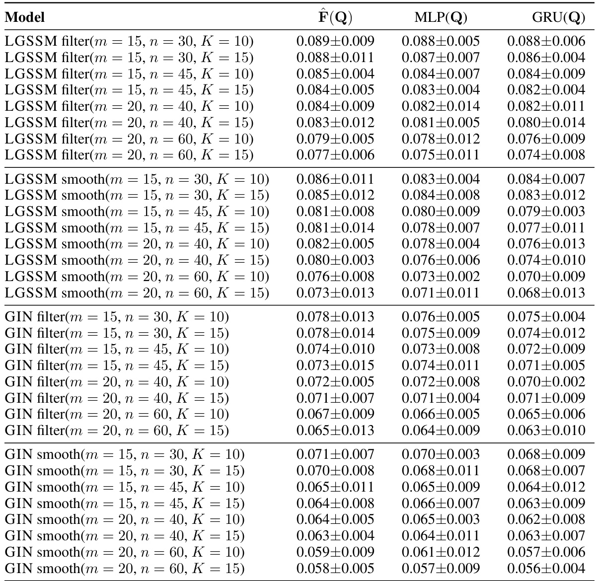
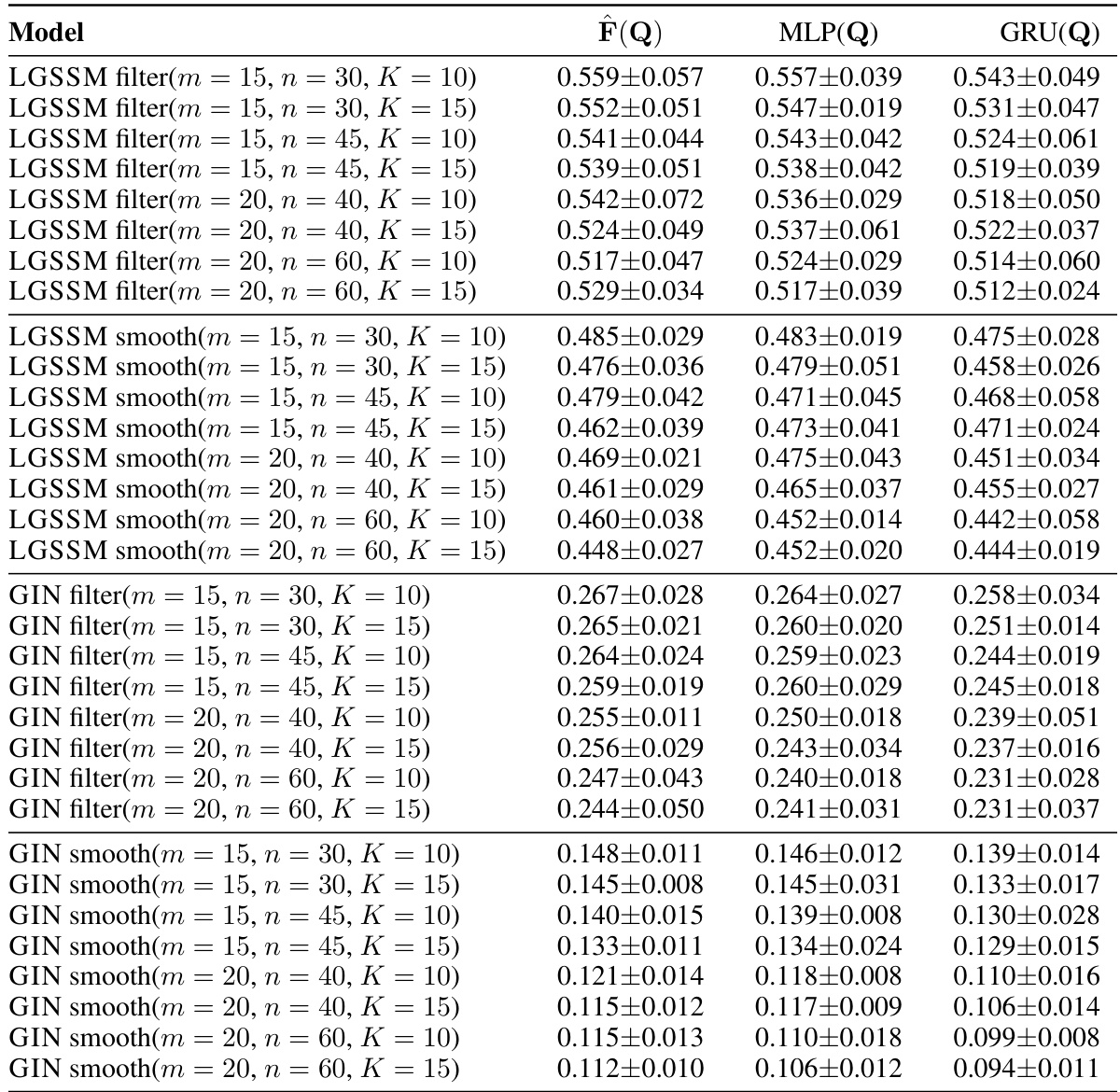
This table shows the Mean Squared Error (MSE) for the double pendulum state estimation task. Different model configurations are compared, varying the number of LSTM/GRU units and the dimension of the observations (m). Each model configuration is evaluated with three different process noise parameterizations (F(Q), MLP(Q), GRU(Q)). The results are useful for comparing the performance of the models under different parameter settings and noise models.

This table presents the results of state estimation experiments conducted on three different systems: a double pendulum, a single pendulum, and a ball in a polygon. It compares the performance of the GIN model to various other methods (VAE, IWVAE, VAE-RNN, SVAE, KVAE, EKVAE, MVAE, DeepAR, RKN, CRU, etc.) by reporting the Squared Error (SE) for the estimated positions of the system’s joints (for the double pendulum) or the ball (for the single pendulum and polygon). The table also shows the log-likelihood achieved by each model. The
svalues represent samples generated based on Equation 10 from the paper.
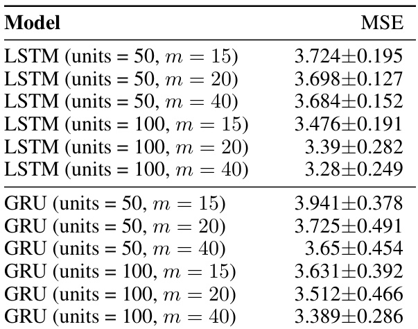
This table shows the Mean Squared Error (MSE) for the bouncing ball experiment, broken down by model and parameter settings. The models tested include LSTMs and GRUs with varying numbers of units and embedding dimensions (m). Different configurations of the Gated Inference Network (GIN), including filtering and smoothing versions with different numbers of states (n) and dynamic clusters (k), are also shown. The results illustrate how different model architectures and hyperparameters affect the accuracy of the state estimation for this complex scenario.
This table presents the state estimation results for three different scenarios: double pendulum, single pendulum, and a ball in a polygon. It compares the Squared Error (SE) and log-likelihood achieved by the GIN model against several other models (VAE, IWVAE, VAE-RNN, etc.). The table shows that the GIN model outperforms other models on this task, particularly achieving the highest log-likelihood in many instances.
Full paper#
