↗ OpenReview ↗ NeurIPS Homepage ↗ Chat
TL;DR#
Neural Collapse (NC), a phenomenon where classifier weights converge to a Simplex ETF, is usually observed after extensive training. Existing methods that leverage NC by fixing classifier weights to a canonical simplex ETF have not shown improvements in convergence speed. This paper introduces a novel mechanism that dynamically finds the nearest simplex ETF geometry to the features at each iteration, addressing this issue by implicitly setting the classifier weights through a Riemannian optimization. This inner-optimization is encapsulated within a declarative node, enabling backpropagation and end-to-end learning.
This method significantly accelerates the convergence to a NC solution, outperforming both fixed simplex ETF approaches and conventional training methods. The approach also enhances training stability by substantially reducing performance variance. Experiments on synthetic and real-world datasets demonstrate superior convergence speed and stability compared to existing methods. The Riemannian optimization problem and its inclusion within a declarative node are key technical contributions that make end-to-end learning feasible. This is a significant advancement for accelerating convergence and improving stability in deep learning models.
Key Takeaways#
Why does it matter?#
This paper is important because it proposes a novel method to accelerate the training of neural networks and improve their stability. It leverages the phenomenon of Neural Collapse, a recently observed characteristic of well-trained networks, to guide the optimization process. This approach could be particularly useful for large-scale deep learning tasks, where training time and stability are major challenges. It provides a new avenue for research in deep learning optimization and offers a practical solution to address convergence issues. The use of Riemannian optimization and deep declarative nodes introduces new techniques to the field.
Visual Insights#

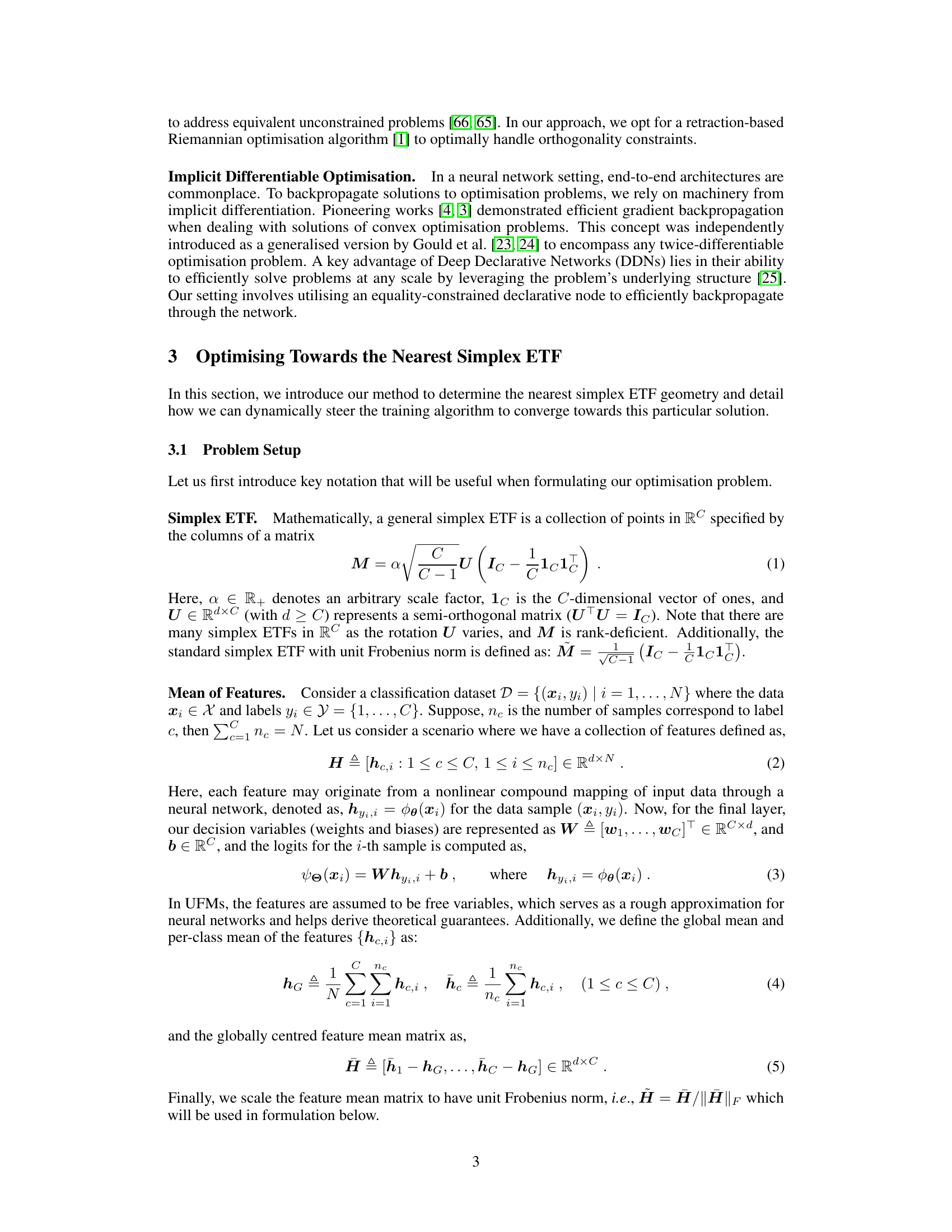
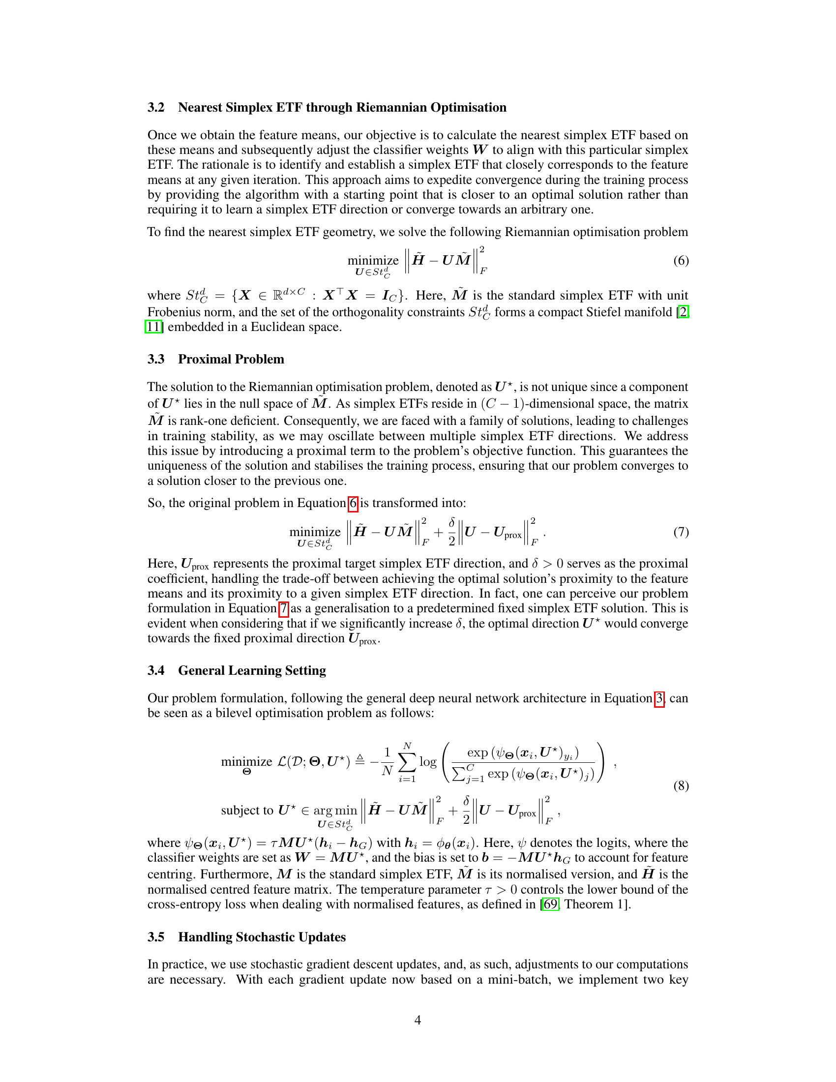
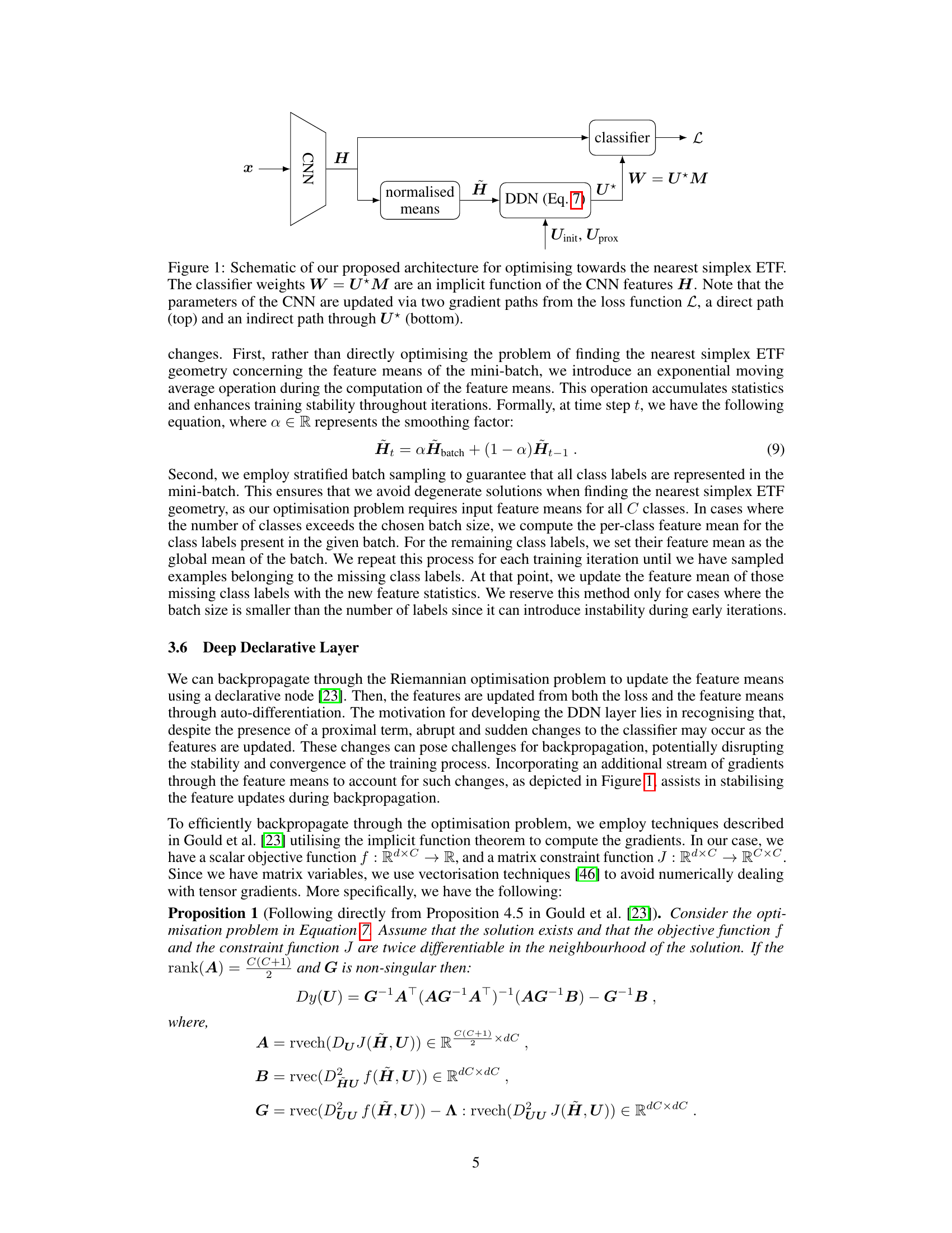
This figure shows the proposed architecture that optimizes towards the nearest simplex ETF. The input x goes through a CNN to produce features H. These features are processed to compute normalized class means which then feeds into a deep declarative network (DDN) that solves for the optimal rotation matrix U*. The classifier weights W are then set implicitly as W = UM, where M is the standard simplex ETF. This is done to efficiently align classifier weights with the features and speed up training. Note that the CNN is updated via gradients from both the loss L and U.

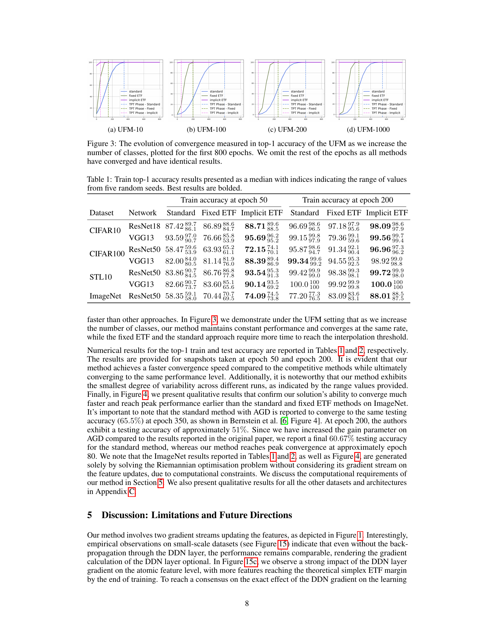
This table presents the top-1 training accuracy results for different neural network models trained on four benchmark datasets (CIFAR-10, CIFAR-100, STL-10, and ImageNet). Three training methods are compared: standard training, fixed simplex ETF, and the proposed implicit ETF method. The results are reported at epochs 50 and 200, showcasing the convergence speed and performance differences between methods. The median accuracy and the range of values across five runs with different random seeds are presented to demonstrate the stability of the method.
In-depth insights#
NC Optimization#
NC optimization, in the context of neural collapse, focuses on accelerating convergence to the optimal solution space characterized by a Simplex Equiangular Tight Frame (ETF). The core idea is to leverage the inherent structure of NC, where classifier weights and penultimate layer feature means converge to a simplex ETF, thereby improving training efficiency and stability. This is achieved by incorporating a mechanism to guide the training process toward the nearest simplex ETF at each iteration, often formulated as a Riemannian optimization problem. This problem is typically solved iteratively within the training loop, allowing for implicit updates to the classifier weights based on the current feature means, often using techniques like implicit differentiation and deep declarative networks to enable efficient backpropagation. Addressing the non-uniqueness of simplex ETF solutions is crucial, often mitigated by regularization methods or proximal terms in the optimization problem. The effectiveness of this approach is demonstrated through faster convergence speed and reduced variance in network performance compared to standard training and fixed-ETF methods. Key challenges include the computational cost of solving the Riemannian optimization, particularly for large-scale networks, and ensuring stability during training.
Simplex ETF Geom#
The concept of “Simplex ETF Geom” likely refers to a geometric representation of Simplex Equiangular Tight Frames (ETFs) within a specific context, perhaps in the context of neural networks. Simplex ETFs are characterized by their optimal weight separation, maximizing the margin between classes. The “Geom” aspect suggests the focus is on the geometrical properties and relationships of these frames. This could involve analyzing the structure of the ETF points, their arrangement in a high-dimensional space, and how these properties relate to the performance of a model, particularly the convergence speed. The analysis might involve tools from Riemannian geometry, dealing with orthogonality constraints inherent in ETF structures. The ultimate goal is likely to leverage the inherent properties of this specific geometric structure, perhaps as a regularization technique, to enhance training stability and convergence in machine learning. Understanding the implications of this geometric structure could lead to new optimization algorithms or improved training techniques for machine learning models.
Riemannian Opt#
The heading ‘Riemannian Opt’ strongly suggests a section detailing the optimization of a problem using Riemannian geometry. This is a powerful mathematical framework for handling optimization problems on curved spaces or manifolds, unlike traditional methods suited for Euclidean spaces. The use of Riemannian optimization techniques implies that the problem’s parameters or variables reside within a non-Euclidean space, necessitating specialized methods. The specific manifold used likely depends on the problem’s constraints. For instance, if dealing with orthogonal matrices, the Stiefel manifold might be involved. Solving the optimization problem requires algorithms designed to operate on Riemannian manifolds. These might include gradient-based techniques adjusted to account for the curvature, or other specialized methods. The approach’s advantage lies in its ability to efficiently address problems with constraints like orthogonality, which are common in machine learning contexts. This section’s deeper analysis should reveal details about the chosen algorithm, its implementation, convergence properties and computational cost within the larger context of the research.
DDN Backprop#
The section on “DDN Backprop” likely details the method for backpropagating gradients through a deep declarative network (DDN) layer. This is crucial because the core of the proposed approach involves implicitly defining classifier weights by solving a Riemannian optimization problem within the DDN. Standard backpropagation techniques cannot directly handle this implicit relationship. The authors probably describe how they encapsulate the Riemannian optimization as a differentiable node, allowing gradients from the loss function to flow backward and update the feature means implicitly influencing the classifier weights. This likely involves techniques from implicit differentiation, enabling end-to-end learning despite the nested optimization. The authors might highlight the efficiency and stability gains of this approach compared to explicitly training the classifier weights, potentially showcasing how it facilitates faster convergence and reduces variance in performance. A key aspect could be the computational efficiency and scalability, given that solving an optimization problem within each backpropagation step could be computationally intensive for large-scale networks. They may discuss strategies for mitigating this computational cost. Furthermore, the details of the implementation within a deep learning framework are likely provided, including specifics on the implementation of the differentiable optimization layer. Finally, the authors may present experimental results to support the claim that their DDN backpropagation approach is effective and offers substantial benefits in training stability and speed.
Future Works#
Future work could explore several promising avenues. Improving the efficiency of the Riemannian optimization within the DDN framework is crucial, especially for large-scale datasets, where computational cost becomes a significant bottleneck. This may involve exploring alternative optimization algorithms or developing more efficient ways to handle the implicit differentiation. Investigating the impact of the DDN gradient backpropagation on different network architectures and datasets will yield valuable insights into the method’s generalizability and effectiveness. A thorough comparison with other state-of-the-art methods for improving neural collapse convergence will further solidify the proposed approach’s position. Additionally, research into theoretical guarantees for the proposed optimization problem is essential to provide a deeper understanding of its convergence behavior and stability. Finally, examining the method’s application to other machine learning problems, such as semi-supervised learning or transfer learning, is a valuable avenue for expanding the scope and impact of the research.
More visual insights#
More on figures
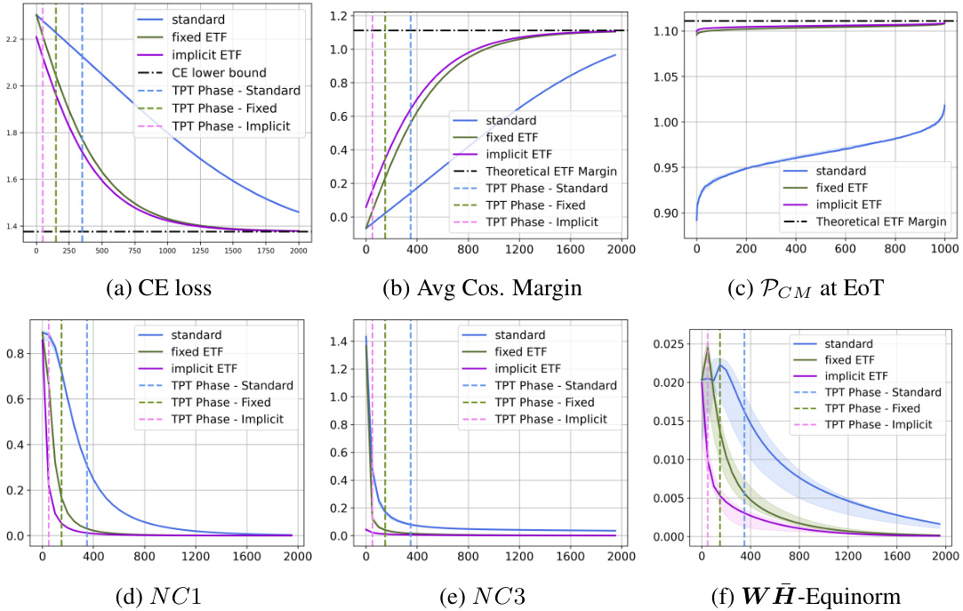
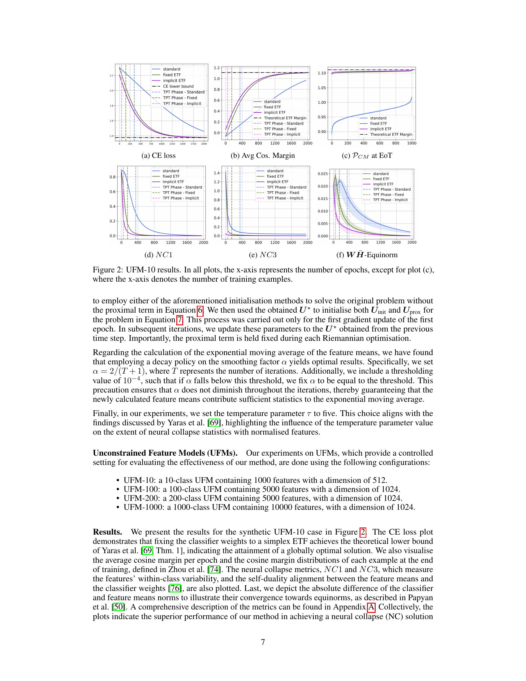
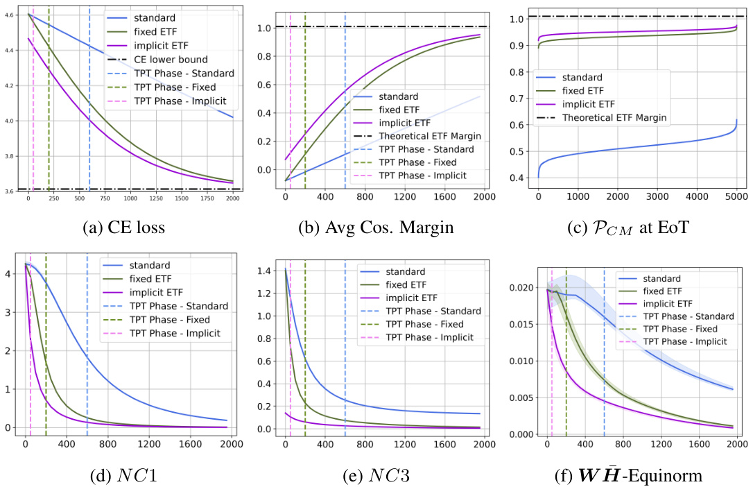
This figure shows the results of the UFM-10 experiment, which evaluates the effectiveness of the proposed method on a 10-class unconstrained feature model (UFM) with 1000 features and a dimension of 512. The plots display various metrics to measure the convergence and performance of different methods: standard training, fixed simplex ETF, and the proposed implicit ETF method. These metrics include cross-entropy (CE) loss, average cosine margin, principal component margin (PCM) at the end of training, Neural Collapse metrics NC1 and NC3, and WH-Equinorm. Each metric’s plot shows the evolution of that metric over training epochs, providing insights into the speed and stability of convergence for each method.

This figure presents the results of the UFM-10 experiment, which is a 10-class unconstrained feature model (UFM) with 1000 features and a dimension of 512. The plots show the performance of three methods: standard training, fixed ETF (equiangular tight frame), and implicit ETF (the method proposed in the paper). The plots cover several metrics: cross-entropy loss, average cosine margin, per-class margin at the end of training, three neural collapse metrics (NC1, NC3, WH-equinorm), illustrating the convergence speed and the quality of the neural collapse solution achieved by each method.
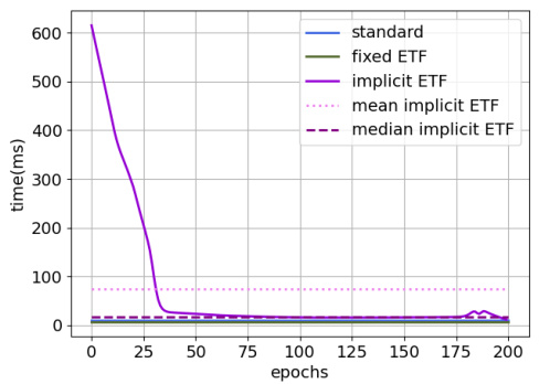
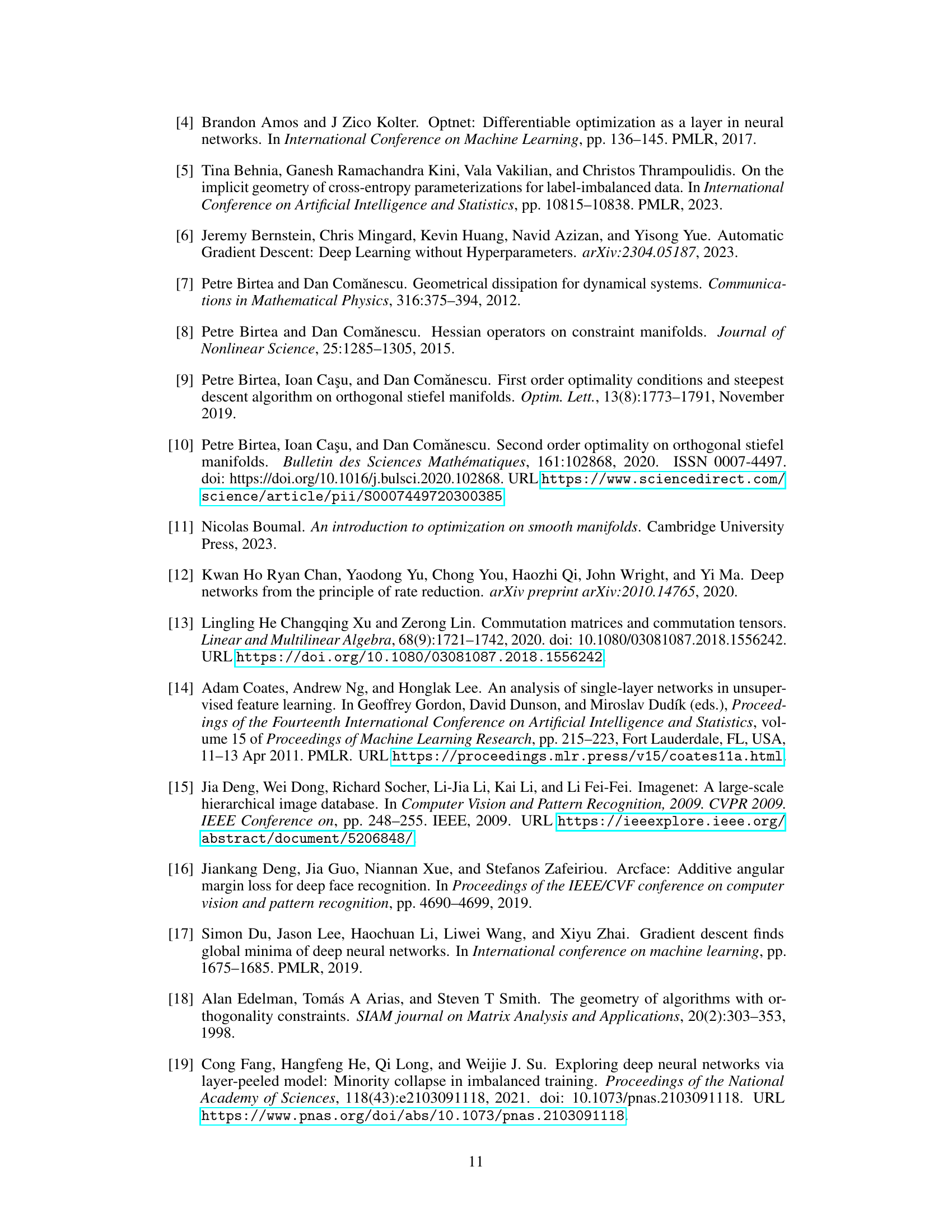
This figure shows the computational cost comparison between different methods in terms of forward and backward pass times. The implicit ETF method, having dynamic computation times, presents both mean and median values. A clear notation explains the meaning of each label.

This figure shows the computational cost of different methods for CIFAR100 dataset on ResNet-50 architecture. The left subplot (a) compares the forward pass time for Standard, Fixed ETF, and Implicit ETF methods. The right subplot (b) displays a comparison of both forward and backward pass times for all methods, illustrating the additional computational overhead introduced by the Implicit ETF method, especially when including backpropagation through the DDN layer.

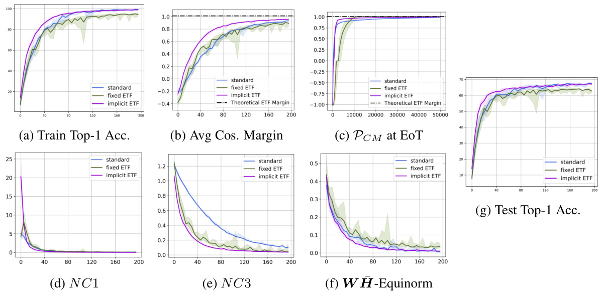
This figure shows the results of the proposed method on CIFAR-10 dataset using ResNet-18 architecture. It presents various metrics (Train Top-1 Accuracy, Average Cosine Margin, Pcm at EoT, NC1, NC3, WH-Equinorm, Test Top-1 Accuracy) across different training epochs, comparing the proposed method against a standard training approach and a fixed ETF approach. The plots illustrate the convergence speed and the final performance of each method, highlighting the superiority of the proposed approach in achieving a neural collapse solution.
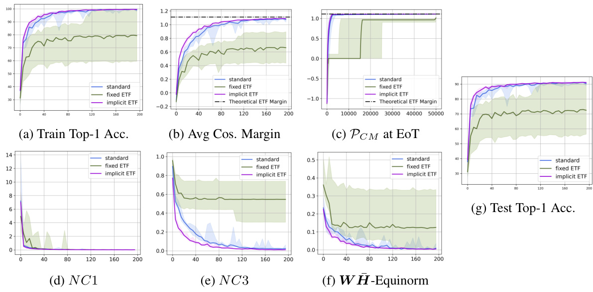
This figure shows the results of experiments on CIFAR10 dataset using ResNet-18 architecture. It presents a comparison of three methods: standard training, fixed ETF, and implicit ETF. Several metrics are plotted against the number of epochs to illustrate the convergence behavior of each method. These metrics include training top-1 accuracy, average cosine margin, per-class mean at end of training (PCM at EoT), NC1 (within-class variability of features), NC3 (alignment of classifier weights and feature means), and WH-Equinorm (equality of norms for feature means and classifier weights). The x-axis represents the number of training epochs for all plots except for the PCM plot where the x-axis shows the number of training examples.

This figure presents the experimental results for CIFAR-10 dataset using ResNet-18 architecture. It displays the training and testing accuracy, average cosine margin, per-class margin at the end of training, neural collapse metrics (NC1, NC3), and the WH-equinorm. The plots show the performance of three methods: standard training, fixed ETF, and implicit ETF (proposed method). The x-axis represents the number of epochs, except for the per-class margin plot (c) where it represents the number of training examples.
This figure shows the results of the UFM-10 experiment, which involves a 10-class unconstrained feature model with 1000 features and a dimension of 512. The plots illustrate the performance of three methods: standard training, fixed ETF, and implicit ETF. The plots show the cross-entropy loss, average cosine margin, per-class mean at the end of training, neural collapse metrics NC1 and NC3, and the WH-equinorm metric. The x-axis represents either the number of epochs (a, b, d, e, f) or the number of training examples (c). These plots show that the implicit ETF method achieves a neural collapse (NC) solution faster than the other two methods.
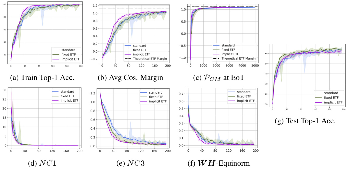
This figure displays the results of the proposed method on the CIFAR10 dataset using the ResNet-18 architecture. It shows the performance of three different training methods: the standard method, the fixed ETF method, and the implicit ETF method (the proposed method). The plots visualize various metrics over the training epochs to evaluate the convergence and performance of each method. These metrics include training and test top-1 accuracy, average cosine margin, per-class margin at the end of training, three Neural Collapse metrics (NC1, NC3, and WH-Equinorm). The plots illustrate that the proposed implicit ETF method converges faster and achieves better performance than the other two methods.

This figure shows the architecture of the proposed method. The Convolutional Neural Network (CNN) extracts features (H) from the input. These features are then processed by a Deep Declarative Network (DDN) that solves a Riemannian optimization problem to find the nearest Simplex Equiangular Tight Frame (ETF) (U*). The classifier weights (W) are implicitly defined as W = U*M, where M is the standard simplex ETF. The gradients are backpropagated through both the CNN and the DDN to update the CNN parameters, facilitating end-to-end learning. The diagram highlights two gradient paths: one direct from the loss function (L) to the CNN and another indirect path through the DDN.
This figure shows the results of the proposed method on a synthetic 10-class unconstrained feature model (UFM) with 1000 data points. The plots display several metrics to assess the effectiveness of the method, comparing it against a standard training approach and a fixed simplex equiangular tight frame (ETF) approach. These metrics include the cross-entropy (CE) loss, average cosine margin, the proportion of correctly classified examples at the end of training, and neural collapse metrics (NC1, NC3). The plots demonstrate that the proposed method converges faster and achieves better performance compared to the other methods.

This figure presents the results of experiments on a 10-class Unconstrained Feature Model (UFM) with 1000 features and a dimension of 512. It displays six subplots illustrating different aspects of the training process using three methods: the standard method (learnable classifier weights), the fixed ETF method (classifier fixed to a predefined simplex ETF), and the implicit ETF method (classifier weights dynamically updated based on the nearest simplex ETF to the features at each iteration). The subplots show the evolution of (a) cross-entropy (CE) loss, (b) average cosine margin, (c) per-class margin at the end of training, (d) neural collapse metric NC1, (e) neural collapse metric NC3, and (f) WH-equinorm. The x-axis represents the number of epochs for plots (a), (b), (d), (e), and (f), while for plot (c), the x-axis represents the number of training examples. The plots demonstrate the superior convergence speed and stability of the proposed implicit ETF method in achieving a neural collapse (NC) solution.

This figure presents the results of the UFM-10 experiment, which involves a 10-class unconstrained feature model with 1000 features and a dimension of 512. It displays six subplots illustrating the performance of three methods: standard training, fixed ETF, and the proposed implicit ETF approach. The plots visualize the evolution of several key metrics over the training epochs, such as cross-entropy (CE) loss, average cosine margin, the proximity to a simplex ETF (PCM) at the end of training, and Neural Collapse metrics (NC1, NC3) indicating the within-class variability of features. The WH-Equinorm plot shows the absolute difference in norms between the classifier and feature means. The results highlight how the proposed method rapidly converges to an optimal neural collapse solution compared to the other two methods.
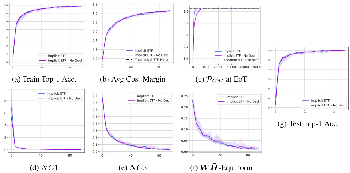
This figure compares the performance of the proposed implicit ETF method with and without the deep declarative network (DDN) layer’s gradient. It shows that the DDN layer’s gradient improves convergence speed and training stability. The plots include training top-1 accuracy, average cosine margin, per-class mean at the end of training, neural collapse metrics (NC1, NC3), within-class and between-class equinorm, and test top-1 accuracy.
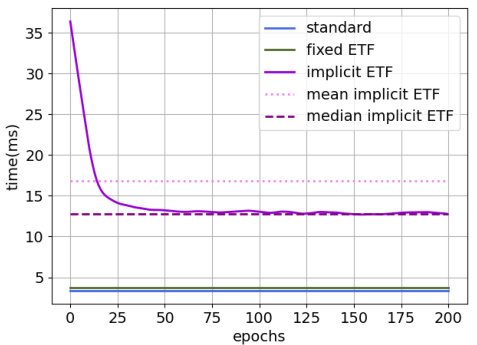
This figure shows the computational cost (forward and backward pass times) of different training methods for CIFAR100 dataset on ResNet-50. The implicit ETF method has dynamic computation times due to the Riemannian optimization, so mean and median values are also provided. The figure helps to understand the efficiency and scalability of the proposed implicit ETF method compared to the standard and fixed ETF methods.

This figure shows the computational cost of different methods (standard, fixed ETF, implicit ETF) on the CIFAR10 dataset using the ResNet-50 architecture. It compares the forward and backward pass times, highlighting the dynamic computation times of the implicit ETF method. The median and mean computation times are shown for the implicit ETF method. The notation used is clearly explained in the caption.
This figure compares the performance of the implicit ETF method with and without the Deep Declarative Network (DDN) layer’s gradient included in the training updates. It shows that the DDN layer’s gradient improves the convergence and performance of the algorithm, but that the implicit ETF method still shows improvements even without DDN gradients. The plots show train and test accuracy, cosine margin, per-class margin, within-class variability, and self-duality metrics.

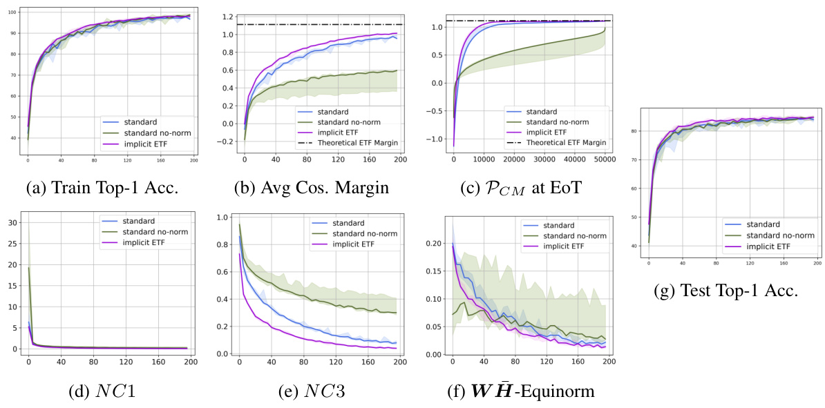
This figure compares the performance of three different training methods on the CIFAR10 dataset using the ResNet-18 architecture. The methods are: standard training (with feature and weight normalization), standard training without normalization, and the proposed implicit ETF method. The plots show various metrics to evaluate convergence to neural collapse, including training accuracy, average cosine margin, per-class margin at end of training, neural collapse metrics (NC1, NC3), weight-feature equinorm, and test accuracy. The results highlight the effectiveness of the implicit ETF method in achieving neural collapse, even when compared to standard training that does not include feature and weight normalization.
More on tables

This table presents the top-1 training accuracy results for different neural network models trained on four benchmark datasets (CIFAR-10, CIFAR-100, STL10, and ImageNet). The results are shown for two different epochs (50 and 200) and for three training methods: Standard, Fixed ETF, and Implicit ETF. The median accuracy and the range of accuracy across five different runs are presented. Bold values indicate the best result for each dataset and epoch.
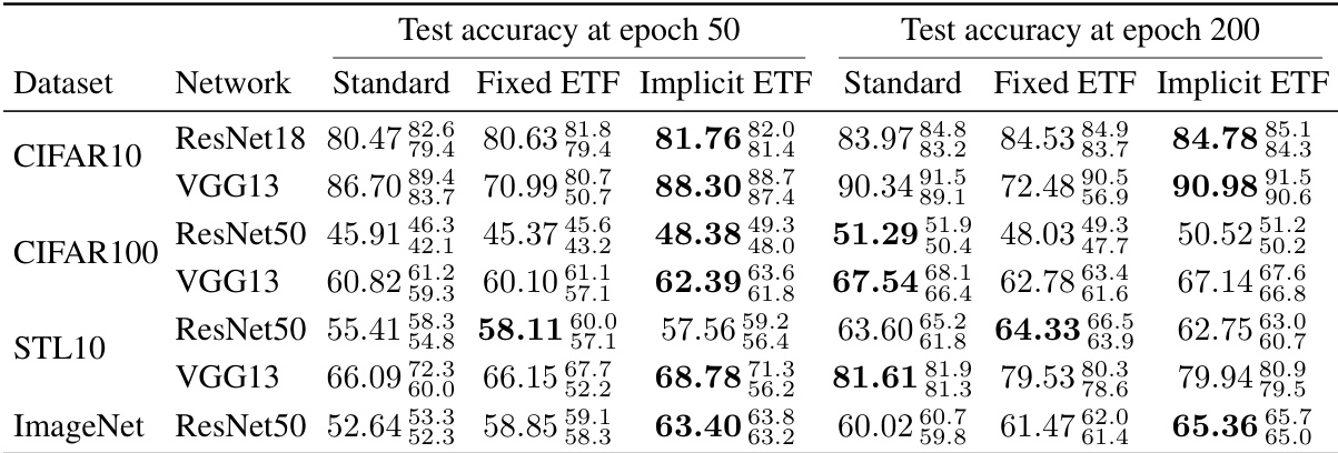
This table shows the training top-1 accuracy results for different neural network models (ResNet18, VGG13, ResNet50) trained on various datasets (CIFAR10, CIFAR100, STL10, ImageNet). The results are presented as median values across five runs with different random seeds, along with the range of values. The table compares three training methods: standard training, fixed ETF, and implicit ETF. The best results for each dataset and network architecture are highlighted in bold.

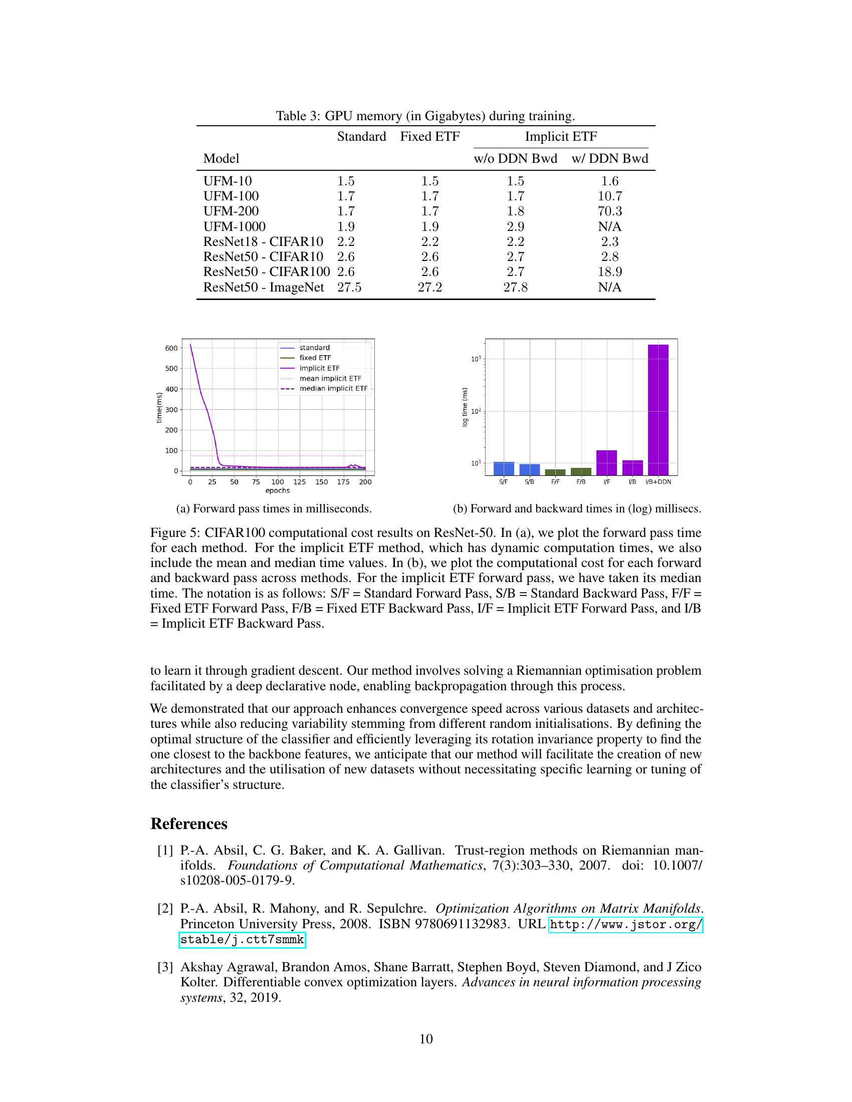
This table shows the GPU memory usage in gigabytes for different models and training methods. It compares the memory consumption of the standard training method, the fixed ETF method, and the implicit ETF method (with and without the DDN backward pass). The models include various UFM sizes (UFM-10, UFM-100, UFM-200, UFM-1000) and several real-world models trained on CIFAR10 and ImageNet datasets using ResNet18 and ResNet50 architectures.
Full paper#
