↗ OpenReview ↗ NeurIPS Homepage ↗ Chat
TL;DR#
Neural population activity often displays distinct dynamic features across time, reflecting internal processes or behavior. Traditional linear methods struggle to capture these complex, non-linear neural dynamics. Existing methods, such as HMMs and SLDS, fail to fully represent neural activity’s intricacy.
This paper introduces Switching Recurrent Neural Networks (SRNNs), a novel approach that reconstructs these dynamics using RNNs with time-varying weights. Applying SRNNs to both simulated and real neural data (from mice and monkeys) enables automatic detection of discrete states linked to varying neural activity. The results show SRNNs successfully capture behaviorally relevant switches and associated dynamics.
Key Takeaways#
Why does it matter?#
This paper is important because it presents a novel approach to understanding neural dynamics using Switching Recurrent Neural Networks (SRNNs). This method addresses limitations of existing techniques by effectively capturing the nonlinear and time-varying nature of neural activity. The findings have significant implications for neuroscience research, opening new avenues for investigating complex brain functions and behaviors. The results also demonstrate the potential of SRNNs to be applied to diverse neurophysiological datasets, showcasing its broad applicability and utility. SRNN is a powerful approach for analyzing neural dynamics and holds promise for furthering our understanding of brain function.
Visual Insights#

This figure shows the architecture of the Switching Recurrent Neural Network (SRNN) model proposed in the paper. Panel A shows a schematic of the SRNN, highlighting the switching mechanism between different RNNs based on discrete hidden states. Panel B illustrates the generative model’s structure, depicting how the hidden states and observations are generated from the RNNs and the switch. Finally, Panel C presents the inference network, illustrating how the model infers the hidden states given the observations. Each panel provides a visual representation of the model’s different components and their interactions.
In-depth insights#
Neural Dynamics#
The study of neural dynamics focuses on understanding the temporal evolution of neural activity and how it gives rise to behavior and cognition. The paper explores this by investigating how neural populations exhibit distinct dynamical features over time, potentially corresponding to different internal states or behavioral phases. Nonlinearity is a crucial aspect, as neural systems are inherently complex and cannot be fully captured by linear models. The use of recurrent neural networks (RNNs) is highlighted for their ability to model these nonlinear dynamics effectively. Switching recurrent neural networks (SRNNs), which allow for transitions between different dynamical regimes, are introduced as a powerful tool for analyzing neural time series data with switching dynamics. The results demonstrate the potential of SRNNs to accurately identify and reconstruct these dynamics across various experimental datasets, thereby offering a robust method for analyzing complex neural activity and understanding its behavioral relevance.
SRNN Model#
The SRNN (Switching Recurrent Neural Network) model presents a novel approach to analyzing neural time-series data by incorporating switching dynamics into recurrent neural networks. Unlike traditional RNNs with fixed weights, SRNNs utilize weights that change over time, reflecting transitions between different dynamical regimes. This allows the model to capture nonlinear and time-varying neural activity, which is crucial for understanding complex brain processes. The use of a Markov process to govern state transitions enables the model to automatically identify discrete states and the corresponding dynamical features within each state. Variational inference is used for model training, offering an efficient way to learn the model parameters. This approach is particularly suitable for datasets where neural activity exhibits distinct patterns corresponding to different behavioral states or cognitive processes, allowing for a more nuanced understanding of neural dynamics compared to traditional methods.
Experimental Tests#
An ‘Experimental Tests’ section in a research paper would detail the empirical evaluation of the proposed methods. This would involve describing the datasets used, including their characteristics (size, type, and any relevant preprocessing). The section should then outline the experimental design, clarifying how the methods were evaluated. Key aspects would include metrics used to quantify performance, such as accuracy, precision, recall, or F1-score, and a clear explanation of how these were calculated. Crucially, it should also describe the statistical methods employed for analysis, such as hypothesis tests or confidence intervals, to determine the significance of observed results. Finally, results would be presented clearly, potentially using visualizations like graphs or tables to illustrate the performance of the proposed methods compared to existing baselines. Robustness checks and error analyses are important components, allowing the researchers to evaluate the sensitivity of their results to parameter choices and dataset variations.
Limitations#
A critical analysis of the limitations section in a research paper is crucial for evaluating the robustness and generalizability of the findings. Identifying limitations demonstrates intellectual honesty and strengthens the paper’s credibility. A thoughtful limitations section should not just list shortcomings, but also explore their potential impact on the conclusions. For instance, were assumptions made that might not always hold true in real-world scenarios? How might these limitations affect the broader applicability of the results? Addressing the limitations section with specific examples and potential avenues for future research greatly enhances its value. A strong limitations section will discuss limitations related to methodology (e.g., sample size, data quality, modeling choices), analysis (e.g., statistical significance, potential biases), and the interpretation of results. A well-written limitations section will also suggest mitigating strategies or future research directions to address the identified limitations.
Future Work#
Future work directions stemming from this research on neural dynamics could involve several promising avenues. Extending the SRNN model to incorporate more complex neural architectures like transformers or graph neural networks could potentially improve accuracy and efficiency in modeling intricate neural interactions. Furthermore, exploring the applicability of SRNNs to diverse neural datasets beyond those considered in this study (e.g., EEG, fMRI) is crucial to assess its generalizability and robustness. Investigating the effects of different hyperparameters and model variations on SRNN performance is needed for optimal tuning and improved reliability. Finally, developing a more comprehensive theoretical framework to understand the learned switching dynamics and their behavioral correlates would enhance interpretability and advance our understanding of the complex relationship between neural activity and behavior.
More visual insights#
More on figures

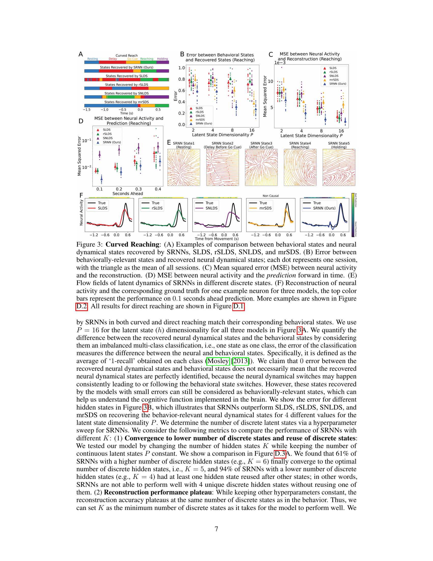
This figure shows the results of applying different models (SRNN, SLDS, rSLDS, SNLDS, mrSDS) to curved reaching data. Panel A shows examples of how well each model aligns the inferred neural dynamical states with the behavioral states. Panel B shows the error between the inferred and actual behavioral states, indicating SRNN’s superior performance. Panel C displays the MSE between the neural activity and its reconstruction by each model. Panel D presents the prediction accuracy of each model. Panel E visualizes the flow fields of the latent dynamics in different discrete states, showcasing their distinct characteristics using SRNN. Finally, panel F compares the neural activity reconstructions for a single neuron across the different models, highlighting SRNN’s accurate reconstruction and prediction.
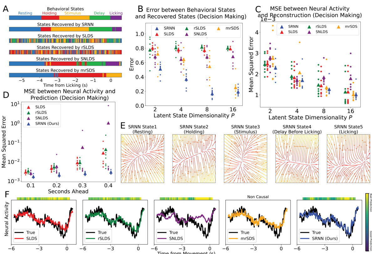
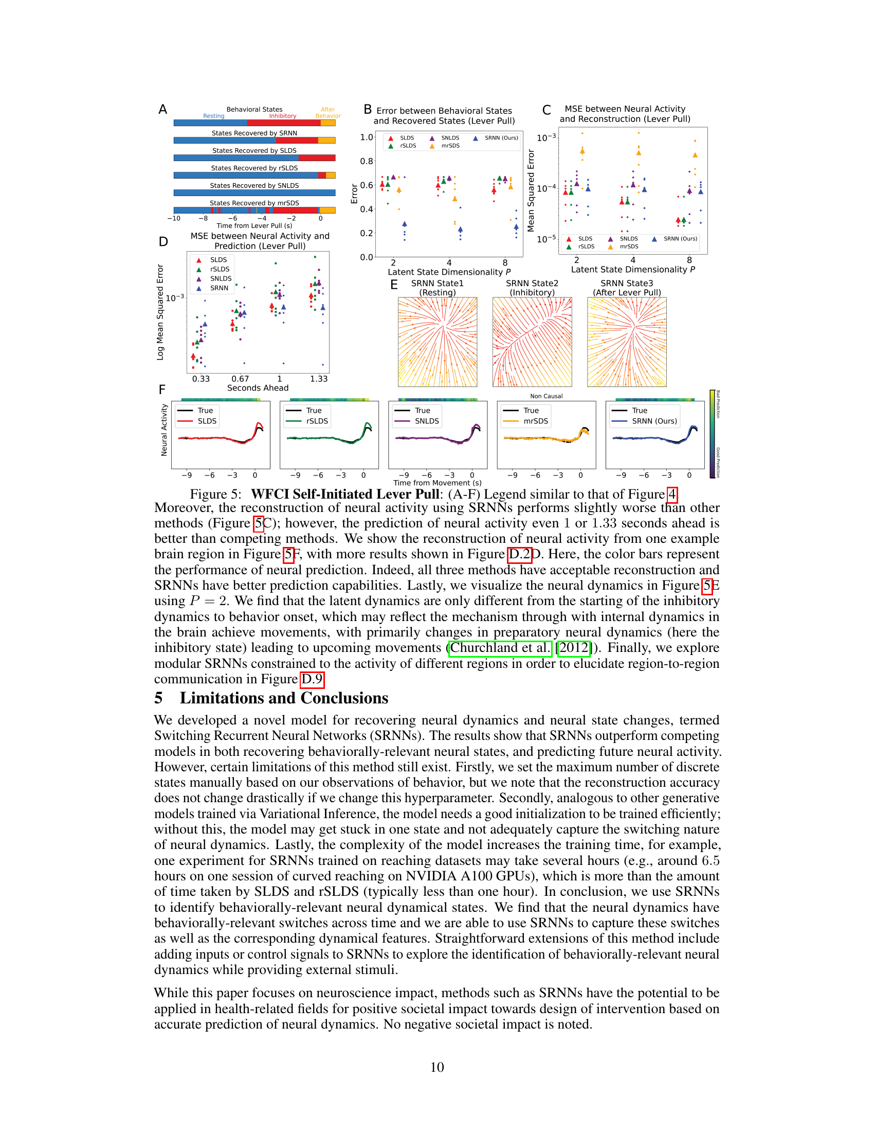
This figure displays the results of applying the Switching Recurrent Neural Network (SRNN) model, along with other competing models like SLDS, rSLDS, SNLDS, and mrSDS, to analyze widefield calcium imaging (WFCI) data from a mouse decision-making task. Panel A shows a comparison between behavioral states and the neural dynamical states identified by each model. Panel B illustrates the error between behavioral states and the recovered states for each model. Panel C depicts the mean squared error (MSE) between the neural activity and the reconstruction for each model. Panel D presents the MSE between the neural activity and the prediction made by each model for different time points into the future. Panel E visualizes the flow fields of latent dynamics in distinct states for the SRNN model. Finally, panel F showcases example neural activity reconstructions by various methods in comparison to the ground truth, with a color bar to show the performance of the 0.33-second ahead predictions. The figure demonstrates the SRNN model’s ability to accurately reconstruct and predict neural activity related to behaviorally-relevant states in a decision making task.

This figure shows a comparison of the performance of SRNNs against other methods (SLDS, rSLDS, SNLDS, and mrSDS) on a monkey reaching task. It visualizes how well each method recovers behavioral states from neural activity and predicts future neural activity, along with the neural dynamics in different discrete states. The figure also includes a reconstruction of neural activity for a single neuron to showcase the performance differences between the models.
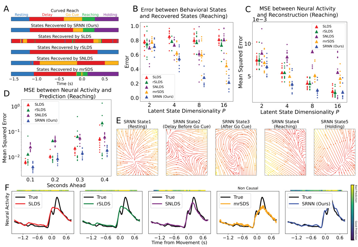
This figure shows a comparison of the performance of SRNNs against other methods for identifying behavioral states from neural activity in a monkey reaching task. Panel A shows examples comparing the recovered neural dynamical states with the actual behavioral states. Panel B quantifies the error between recovered and actual behavioral states. Panel C and D show mean squared error (MSE) for reconstruction and prediction, respectively. Panel E displays the flow fields of the latent dynamics in each discrete state of the SRNN. Panel F shows reconstruction vs ground truth for a single neuron, illustrating prediction accuracy.

This figure demonstrates the performance of Switching Recurrent Neural Networks (SRNNs) on a simulated Lorenz attractor dataset. Panel A shows the high accuracy of SRNNs in reconstructing the simulated data, with the SRNN reconstruction almost perfectly overlapping the ground truth. Panel B compares the ground truth discrete states with those recovered by the SRNN model, highlighting the model’s ability to accurately identify the discrete states. Finally, Panel C visualizes the latent dynamics within each discrete state, showcasing the model’s successful recovery of the underlying dynamical features of the system.

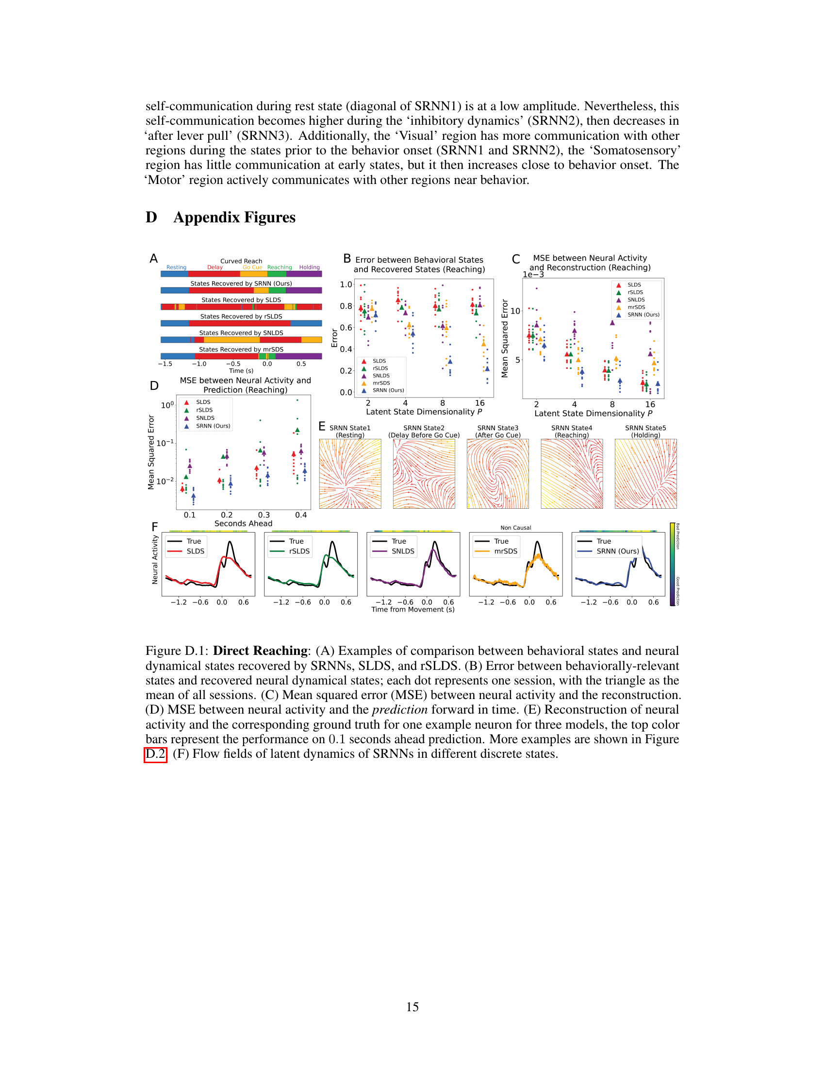
This figure shows a comparison of the performance of SRNNs, SLDS, and rSLDS on a direct reaching task. Panel A displays examples of the comparison between behavioral states and the neural dynamical states recovered by each model. Panel B shows the error between behavioral states and recovered states for each session. Panel C presents the mean squared error (MSE) between the neural activity and the reconstruction for each model. Panel D shows the MSE between neural activity and predictions made 0.1 seconds into the future. Panel E shows the reconstruction of neural activity and the corresponding ground truth for a single neuron. Finally, Panel F illustrates the flow fields of latent dynamics in different discrete states recovered by SRNNs.

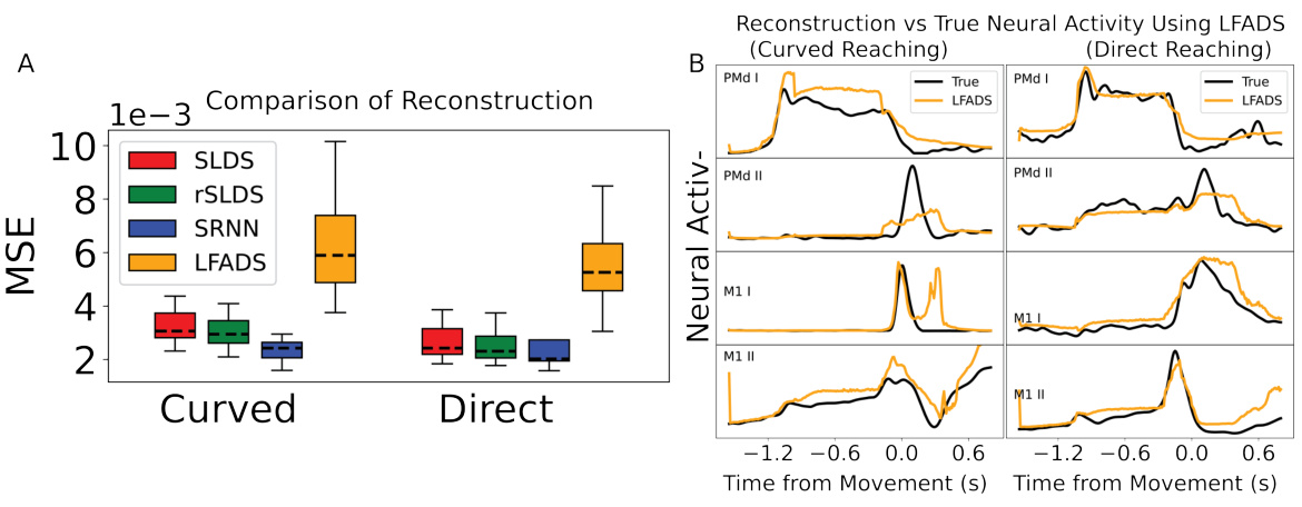
This figure displays the reconstruction of neural activity by different models (SLDS, rSLDS, SNLDS, mrSDS, and SRNN) compared to the true neural activity for four different tasks: curved reaching, direct reaching, self-initiated decision-making, and self-initiated lever pull. Each subfigure shows the true neural activity and the reconstructed neural activity for several example neurons from different brain regions. The color coding helps to distinguish between the different models in the reconstructions.

This figure shows the reconstruction of neural activity by four different models: SLDS, rSLDS, SNLDS, and mrSDS, compared to the ground truth. The reconstruction is shown for four different tasks: curved reaching, direct reaching, self-initiated decision making, and self-initiated lever pull. Different colors represent different models. The figure helps visualize how well each model reconstructs the neural activity for each task and brain region.

This figure shows the results of applying the Switching Recurrent Neural Network (SRNN) model with different numbers of discrete hidden states (K=4, 5, and 6) to curved reaching data. Panel A visually compares the behavioral states with the neural dynamical states recovered by the SRNN for each value of K. Panels B and C show the mean squared error (MSE) between the neural activity and the SRNN reconstruction, with Panel C specifically using a ‘co-smoothing’ technique to address potential issues with the model’s learning process. Panel D presents the variance in behavioral states identified by the SRNN for different values of K. The overall goal of this figure is to show how the choice of K affects the model’s performance in reconstructing neural dynamics and identifying behaviorally relevant states.

Figure D.4 shows the result of applying the Switching Recurrent Neural Network (SRNN) model with different numbers of discrete hidden states (K=4, 5, and 6) to the widefield calcium imaging (WFCI) data from a decision-making task. The figure compares the model’s performance in reconstructing the neural activity (MSE), aligning with behavioral states (error), and the variability of the recovered behavioral states. This helps determine the optimal number of states for the SRNN model.
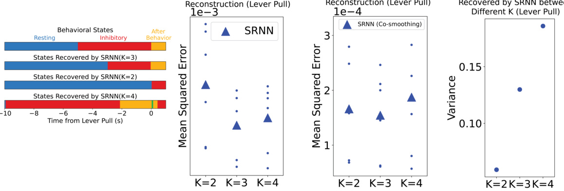
This figure displays the results of applying Switching Recurrent Neural Networks (SRNNs) with varying numbers of discrete states (K) to widefield calcium imaging (WFCI) data from a mouse self-initiated lever pull task. It shows a comparison between behavioral states and the neural dynamical states recovered by the model, mean squared errors (MSE) for different numbers of states, MSEs after applying a ‘co-smoothing’ technique to reduce noise, and the variance of behavioral states across runs. The goal is to determine the optimal number of discrete states for the SRNN model on this particular dataset.
This figure demonstrates the performance of the Switching Recurrent Neural Network (SRNN) model on a simulated Lorenz attractor dataset. Panel A shows the reconstruction of the simulated data using the SRNN model, almost perfectly overlapping the ground truth. Panel B compares the ground truth discrete states to those recovered by the SRNN model, indicating a high degree of accuracy. Finally, Panel C visualizes the latent dynamics within each discrete state, showcasing the model’s ability to capture the underlying dynamical features.

This figure shows the training loss, reconstruction error (MSE), and discrete state recovery error during training of SRNNs on three different datasets: monkey reaching task, mouse self-initiated lever pull task, and mouse self-initiated decision making task. Each column represents a different metric across 5000 training epochs, displayed for each dataset. The plot illustrates the convergence of SRNNs on each task and provides insight into their training dynamics.

This figure compares the performance of SRNNs, SLDS, and rSLDS models on a monkey reaching task. Panel A shows examples of the comparison between behavioral and neural dynamical states. Panel B quantifies the error between recovered states and behavioral states across sessions. Panel C displays the MSE between reconstructed and actual neural activity. Panel D shows the MSE for neural activity prediction. Panel E illustrates an example neuron’s activity reconstruction and ground truth, showing predictive capabilities. Finally, Panel F visualizes the neural dynamics’ flow fields in different discrete states.

This figure shows the results of applying the Switching Recurrent Neural Network (SRNN) model to a simulated Lorenz attractor dataset. Panel A demonstrates the SRNN’s ability to accurately reconstruct the simulated data, almost perfectly overlapping the ground truth. Panel B compares the discrete states identified by the SRNN model against the ground truth, demonstrating a high degree of accuracy in state identification. Finally, Panel C visualizes the latent dynamics within each of the discrete states, revealing the successful recovery of the underlying dynamical features by the SRNN model.
Full paper#
