↗ OpenReview ↗ NeurIPS Homepage ↗ Chat
TL;DR#
Deep learning has shown promise in learning to perform algorithms. However, existing approaches like Deep Thinking (DT) networks often suffer from instability during training and lack guarantees of convergence. This instability significantly limits their applicability to more complex problems. The unreliability of DT networks in extrapolating to unseen data further restricts their capabilities.
This paper introduces Deep Thinking with Lipschitz Constraints (DT-L), a novel approach that addresses these shortcomings. DT-L incorporates Lipschitz constraints into the model’s design, which guarantees convergence during inference. This leads to increased model stability and superior extrapolation performance on more complex tasks. Empirical results show DT-L’s effectiveness in learning and extrapolating algorithms for different problem domains, including the challenging Traveling Salesperson Problem where prior methods failed.
Key Takeaways#
Why does it matter?#
This paper is important because it addresses the instability issues in existing Deep Thinking (DT) networks for algorithm learning. By introducing Lipschitz constraints, it enhances the reliability and stability of DT networks, enabling them to learn and extrapolate to more complex problems than previously possible. This opens new avenues for algorithm learning and algorithm synthesis research. It is highly relevant to current research trends focusing on reliable and stable deep learning models, and its theoretical guarantees of convergence are significant.
Visual Insights#

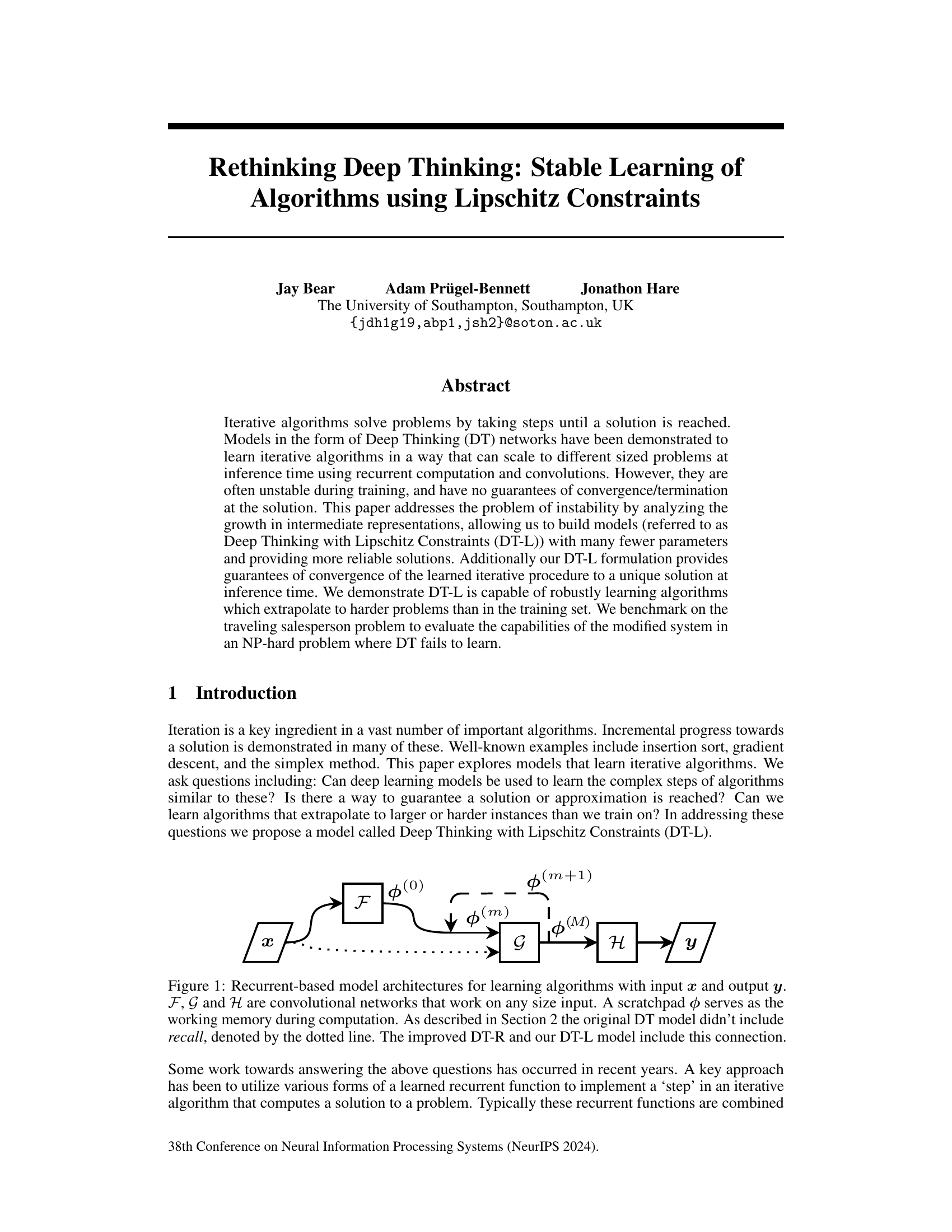
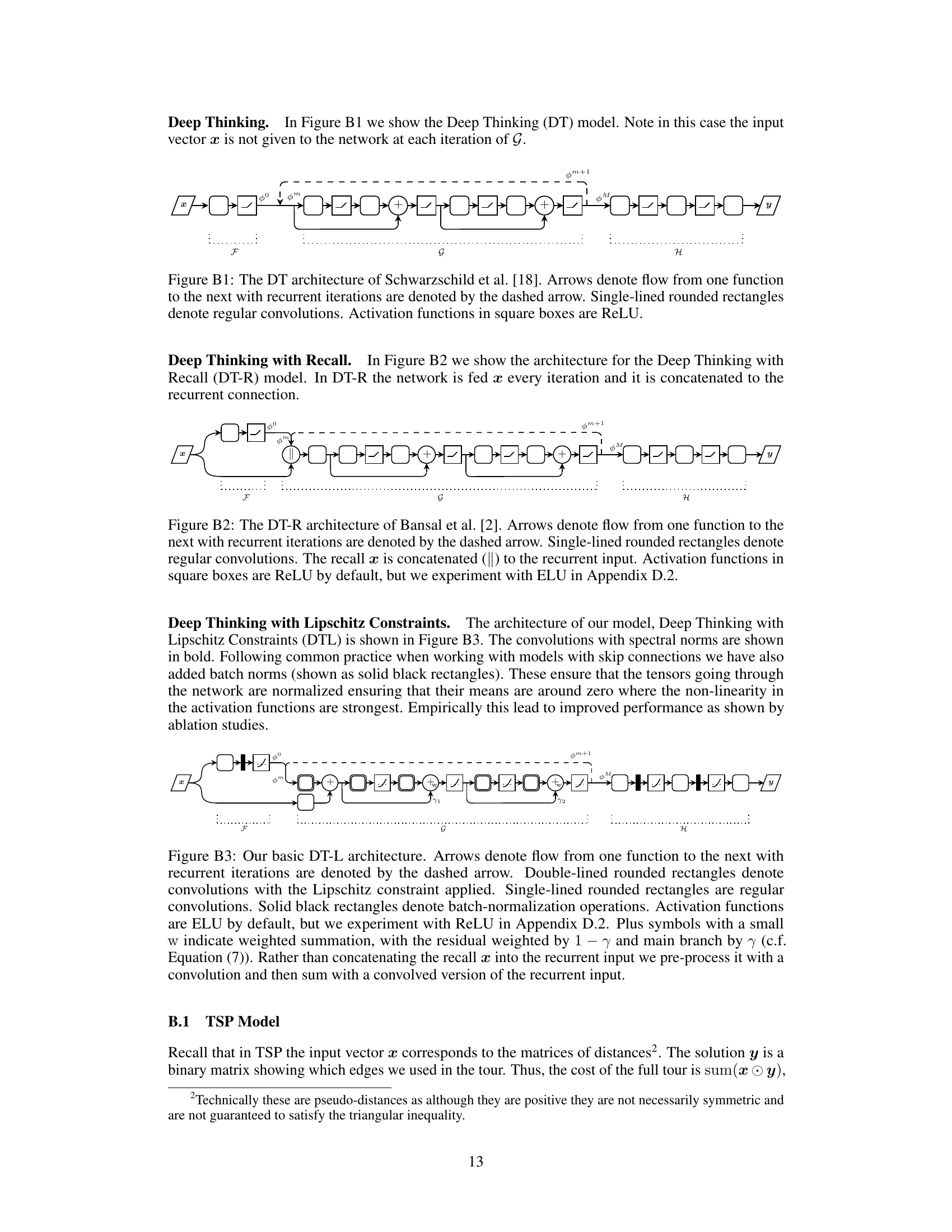
This figure shows three different model architectures used for learning algorithms. The input is represented by ‘x’ and the output by ‘y’. The models use convolutional networks (F, G, H) and a scratchpad (Φ) to store intermediate computations. The key difference between the models is the inclusion of ‘recall’ (dotted line), a connection from the original input ‘x’ to the recurrent function G, which is present in DT-R and DT-L but absent in the original DT model. This allows the model to access the original input throughout the iterative process.

This table presents the results of the Traveling Salesperson Problem (TSP) experiments. It compares the average tour length obtained by the DT-L model against three baselines: random tours, nearest neighbor (NN) tours starting from a random point, and the best nearest neighbor (BNN) tour among all starting points. The comparison is done for both symmetric and asymmetric TSP instances with different numbers of cities (n=15 and n=30). For DT-L, different numbers of iterations (M=45 for n=15, M=120 for n=30) were used. The results show that DT-L significantly outperforms random tours and achieves tour lengths comparable to the NN and BNN baselines, demonstrating the model’s ability to learn effective TSP solving strategies.
In-depth insights#
Stable Algorithm Learning#
Stable algorithm learning, a crucial aspect of machine learning, focuses on developing algorithms that consistently converge to a solution and exhibit robustness against various factors. Instability during training, a major challenge in existing deep learning models like Deep Thinking networks, often leads to unreliable solutions. This is addressed by analyzing the growth of intermediate representations, enabling the construction of models with fewer parameters and improved reliability. Lipschitz constraints are a key technique, guaranteeing convergence to a unique solution at inference time and enhancing the algorithm’s ability to generalize to unseen problems. The effectiveness is demonstrated by successfully learning algorithms that extrapolate to harder problems than those in the training set, showcasing the potential of stable algorithm learning to solve complex problems like the traveling salesperson problem where traditional methods fail.
Lipschitz Constraints#
The concept of Lipschitz constraints, applied within the context of training deep learning models for iterative algorithms, offers a compelling approach to enhance stability and reliability. By imposing a Lipschitz constraint on the recurrent function, the authors aim to control the growth of intermediate representations, preventing issues like exploding gradients during training and ensuring convergence to a unique solution during inference. This constraint acts as a regularizer, limiting the magnitude of changes in the model’s internal state at each iteration and thus promoting stable learning dynamics. Guaranteeing convergence is a significant advantage, particularly for tasks where the iterative process’s termination condition is critical. Furthermore, the use of Lipschitz constraints allows for simpler model architectures with fewer parameters, reducing computational cost and mitigating overfitting. The authors’ analysis of existing deep learning models for algorithms reveals that the lack of such constraints contributes to their instability, highlighting the importance of this modification for improved performance and robustness.
DT-L Model Analysis#
A thorough analysis of the DT-L model would involve a multifaceted approach, examining its architecture, training stability, and performance across various tasks. Architectural analysis would dissect the model’s components, specifically focusing on the modifications implemented to address DT-R limitations. This might include a comparison of the number of parameters, computational complexity, and differences in the convolutional network layers. The introduction of Lipschitz constraints is a key feature; examining how these constraints are imposed, their impact on model capacity and expressiveness, and the trade-off between stability and accuracy is crucial. Training stability analysis would compare DT-L with its predecessors, investigating its resistance to vanishing or exploding gradients, along with assessing its convergence properties through metrics such as training loss and the spectral norm of weight matrices. Finally, a performance analysis would assess the model’s ability to generalize to unseen data through benchmark tests on various problems, comparing its accuracy and extrapolation capabilities to DT and DT-R. Exploring the influence of hyperparameters, such as the Lipschitz constant and choice of activation function, on DT-L’s performance across diverse tasks is also important. Overall, the analysis should rigorously evaluate whether DT-L achieves its goals of enhanced stability, improved extrapolation performance, and efficient use of parameters, providing a comprehensive understanding of its strengths and weaknesses.
Extrapolation Limits#
The concept of “Extrapolation Limits” in the context of machine learning models trained to learn algorithms is crucial. It refers to the boundary beyond which the model’s ability to generalize from smaller, simpler training instances to larger, more complex, unseen instances breaks down. Successful extrapolation is vital for the practical applicability of such learned algorithms, as it allows the model to handle problems outside the scope of its training data. Understanding and defining these limits is key to developing robust models. Factors influencing extrapolation limits include the complexity of the algorithm itself, the choice of model architecture (e.g., the role of recurrent layers or scratchpad memory), and the training strategy employed. Instability during training, frequently observed in deep learning models, can severely restrict extrapolation capabilities. By addressing training instability and incorporating mechanisms such as Lipschitz constraints, we can potentially push extrapolation limits and enable models to solve significantly larger and more complex problems than previously possible. However, there will always be a point where the generalization fails; investigating this failure point is crucial to improve the robustness and wider applicability of this promising area of research.
TSP Benchmark#
The TSP benchmark section would be crucial in evaluating the proposed DT-L model’s performance on a well-known NP-hard problem. It would likely involve generating various TSP instances with different characteristics (symmetric/asymmetric, Euclidean/non-Euclidean, varying number of cities) to test the model’s ability to find near-optimal solutions. The results could be compared to existing algorithms (e.g., approximation algorithms like Christofides’ algorithm, or heuristics like nearest neighbor) demonstrating DT-L’s effectiveness and scalability. Key metrics such as the tour length (average, best, worst) and the time complexity of finding a solution should be reported. The benchmark’s success lies in rigorously demonstrating the model’s ability to learn and extrapolate to solve complex instances not seen during training, highlighting the generalization capability of the DT-L architecture. A comprehensive comparison against established methods would provide a strong validation of the proposed approach’s practical value for solving real-world TSP problems. Failure cases and their analysis would also be important to demonstrate the model’s limitations and to guide future improvements.
More visual insights#
More on figures

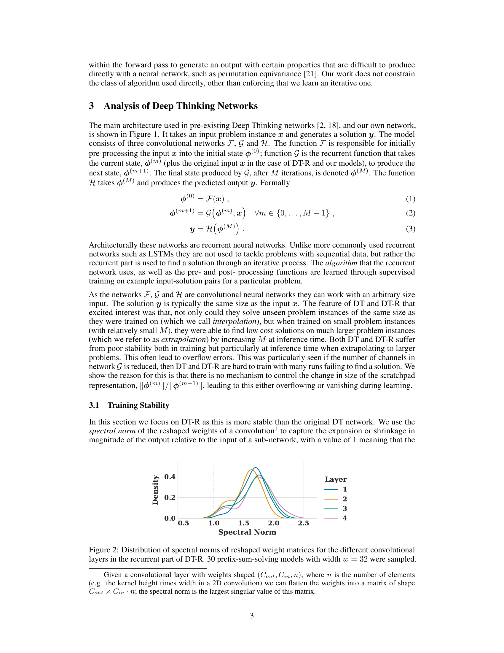
This figure shows the distribution of spectral norms for the convolutional layers in the recurrent part of the DT-R model. The spectral norm is a measure of how much the magnitude of the output of a layer changes relative to its input; a value of 1 indicates no change. The violin plots show the distribution across 30 different prefix-sum solving models (width=32). The plot indicates that in most cases, the spectral norm is greater than 1, meaning the magnitude of the activations increases as it passes through each layer. This contributes to instability in the training and extrapolation behavior of the DT-R model.

This figure shows the training stability of Deep Thinking with Recall (DT-R) models for solving prefix sums problems with varying model widths (w). It plots the mean cross-entropy loss across 10 different model initializations at each training epoch for widths w = 16, 32, 64, 128, and 256. Narrower models (small w) exhibit more stable training, although convergence isn’t guaranteed, while wider models show a higher likelihood of reaching a low loss but also experience significant instability and even model failure (NaN loss) due to loss spikes.

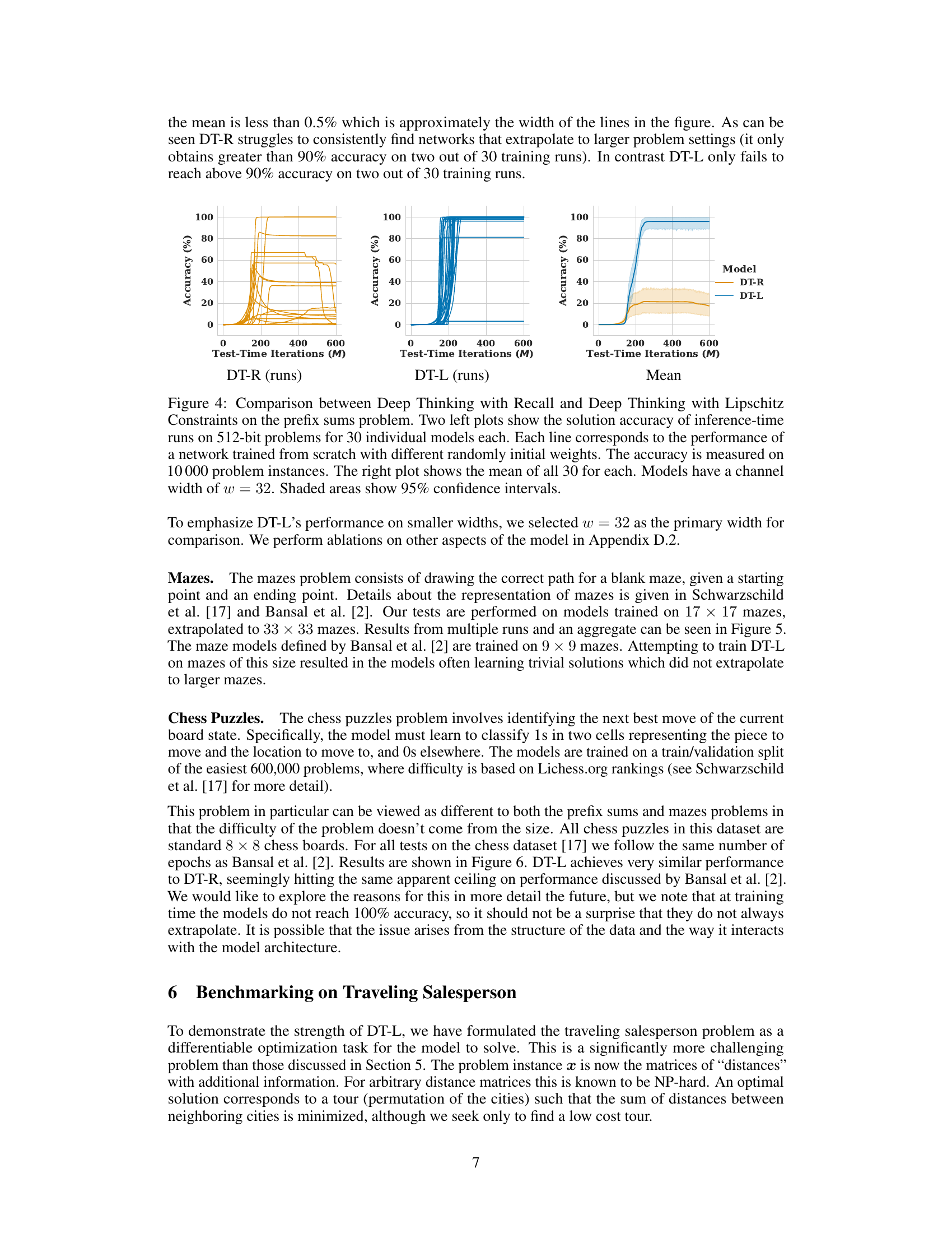
This figure compares the performance of two models, DT-R and DT-L, on the prefix sums problem. DT-R shows unstable performance across multiple runs, with some models failing to reach high accuracy, while DT-L demonstrates much more consistent and reliable performance, achieving high accuracy across nearly all runs. The rightmost plot shows the mean accuracy for each model, highlighting the significant improvement in stability and accuracy provided by DT-L.

This figure compares the performance of two different models, DT-R and DT-L, on the prefix sums problem. The left two plots show the accuracy of 30 different models for each architecture, trained with different random initial weights. The right plot displays the mean performance for each architecture. DT-L demonstrates better and more consistent accuracy across all models. The shaded areas represent 95% confidence intervals.

This figure compares the performance of Deep Thinking with Recall (DT-R) and Deep Thinking with Lipschitz Constraints (DT-L) models on a prefix sum problem. Thirty models of each type were trained independently from random initializations. The left plots show the accuracy of each model on 512-bit test instances, plotted against the number of test-time iterations. The right plot presents the average accuracy for each model type. The results show DT-L’s improved stability and accuracy on larger problems.

This figure shows three different model architectures for learning algorithms. The input is x, and the output is y. All models use convolutional neural networks (F, G, H) that can handle variable-sized inputs. A scratchpad (phi) acts as a working memory. The main difference between the models is how they handle recall of the original input. The original Deep Thinking (DT) model did not include recall, while the Deep Thinking with Recall (DT-R) and Deep Thinking with Lipschitz Constraints (DT-L) models do.

This figure shows three different recurrent neural network architectures used for learning algorithms. The input x is processed by a convolutional network F to produce an initial state. This state is iteratively updated by another convolutional network G (with the original input x also included in DT-R and DT-L). The updated state is further processed by a final convolutional network H to produce the output y. The scratchpad φ represents working memory during this iterative process. The differences between DT, DT-R, and DT-L lie in the inclusion (DT-R and DT-L) or exclusion (DT) of a connection from the original input x to the state update function G, which is represented by a dotted line in the diagram. This ‘recall’ mechanism is a key improvement.

This figure shows three different recurrent neural network architectures for learning algorithms. The input is denoted by ‘x’ and the output by ‘y’. The networks use convolutional layers (F, G, H) and a scratchpad (φ) to store intermediate computations. The key difference between the three architectures is the incorporation of ‘recall’. The original DT model lacks recall, while the improved DT-R and the proposed DT-L model both include a recall connection (dotted line in DT-R, solid line in DT-L), allowing the network to access the original input at each iteration.

This figure shows three different model architectures for learning algorithms. The input is x, and the output is y. The models use convolutional neural networks (F, G, and H) and a scratchpad (φ) to store intermediate results. The key difference between the models is the inclusion or exclusion of a ‘recall’ connection (dotted line). The original Deep Thinking (DT) model lacked recall, while the improved Deep Thinking with Recall (DT-R) and the Deep Thinking with Lipschitz Constraints (DT-L) models include it. This connection allows the models to use the original input (x) at every iteration, which improves performance.

This figure shows the mean training loss for prefix-sum solving models with different widths (w). Each line represents the average training loss across 10 models, each initialized randomly. The dotted vertical lines highlight points where the training loss becomes NaN (Not a Number) or infinite, indicating model failure. The figure extends the results shown in Figure 3 of the main paper, providing additional data points to illustrate the effect of model width on training stability for Deep Thinking with Recall models.

This figure compares the performance of Deep Thinking with Recall (DT-R) and Deep Thinking with Lipschitz Constraints (DT-L) models on the mazes problem. Smaller models (width w=32) were trained on smaller mazes (17x17) and then tested on larger mazes (33x33) to evaluate their ability to extrapolate. The plots show the solution accuracy for 14 different model runs on the larger mazes, with different iterations (M) at inference time. The right-hand plot shows the average accuracy across these 14 runs. Shaded areas represent 95% confidence intervals.

This figure compares the performance of Deep Thinking with Recall (DT-R) and Deep Thinking with Lipschitz Constraints (DT-L) models on a prefix sum problem. The left two subplots show the accuracy of 30 independently trained DT-R and DT-L models on 512-bit test instances, illustrating the variability in model performance. The right subplot shows the average accuracy across all 30 models for both DT-R and DT-L. The shaded regions represent 95% confidence intervals. This figure highlights DT-L’s improved stability and performance compared to DT-R in solving larger problem instances.

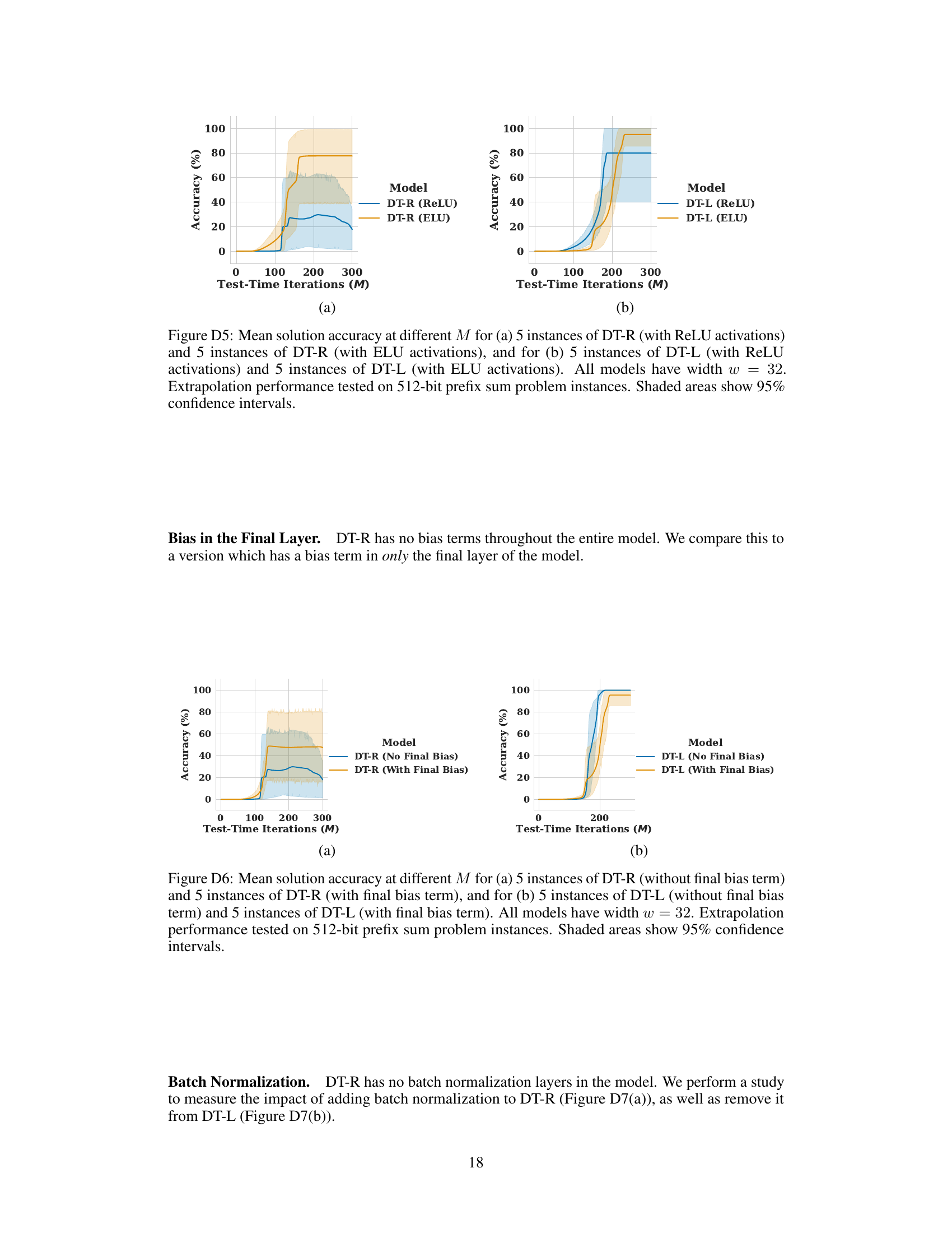
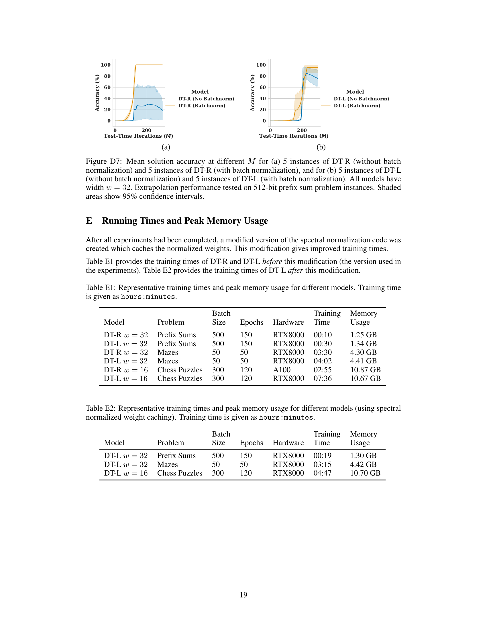
This figure compares the performance of DT-R and DT-L models with and without batch normalization on the prefix sum task. The x-axis represents the number of iterations (M) at inference time, while the y-axis shows the solution accuracy. The shaded regions indicate the 95% confidence intervals. The results demonstrate the impact of batch normalization on model stability and accuracy in extrapolating to larger problems.
More on tables

This table presents the training time and peak memory usage for different models used in the experiments. The models are trained on different problems (Prefix Sums, Mazes, Chess Puzzles) with varying widths (w). Training times are provided in hours:minutes, and peak memory usage is given in GB. The hardware used for training is also specified.

This table shows the training time and peak memory usage for different models used in the paper. The spectral normalized weights are cached to improve training time. The models are trained for different problems such as prefix sums, mazes, and chess puzzles, and the training time and memory usage are measured for each model.

This table shows the training time and peak memory usage for different models trained using spectral normalized weight caching. The models were trained for three different problems (Prefix Sums, Mazes, and Chess Puzzles). The table includes the model’s width (w), the problem type, the batch size, the number of epochs, the hardware used, the training time (in hours and minutes), and the peak memory usage (in GB).

This table presents the training time and peak memory usage for different models trained on various problems (Prefix Sums, Mazes, Chess Puzzles). The models are categorized by type (DT-R and DT-L) and width (w). Training times are given in hours and minutes, while memory usage is in GB. The table helps to compare the computational efficiency of the different models and their ability to scale to more complex problems.

This table presents the training time and peak memory usage for different models using the Deep Thinking with Lipschitz Constraints (DT-L) model, with spectral normalized weight caching. The results are categorized by model (width w), problem type (Prefix Sums, Mazes, Chess Puzzles), batch size, number of epochs, hardware used (RTX8000), training time (in hours:minutes), and peak memory usage (in GB).
Full paper#
