↗ OpenReview ↗ NeurIPS Homepage ↗ Hugging Face ↗ Chat
TL;DR#
Video frame interpolation (VFI) aims to generate intermediate frames between existing ones, crucial for applications like video compression and novel view synthesis. However, accurately modeling motion in real-world videos, with various speeds and occlusions, has been challenging. Existing methods either linearly combine bidirectional flows or directly predict flows for discrete timesteps, lacking the ability to effectively model complex spatiotemporal dynamics.
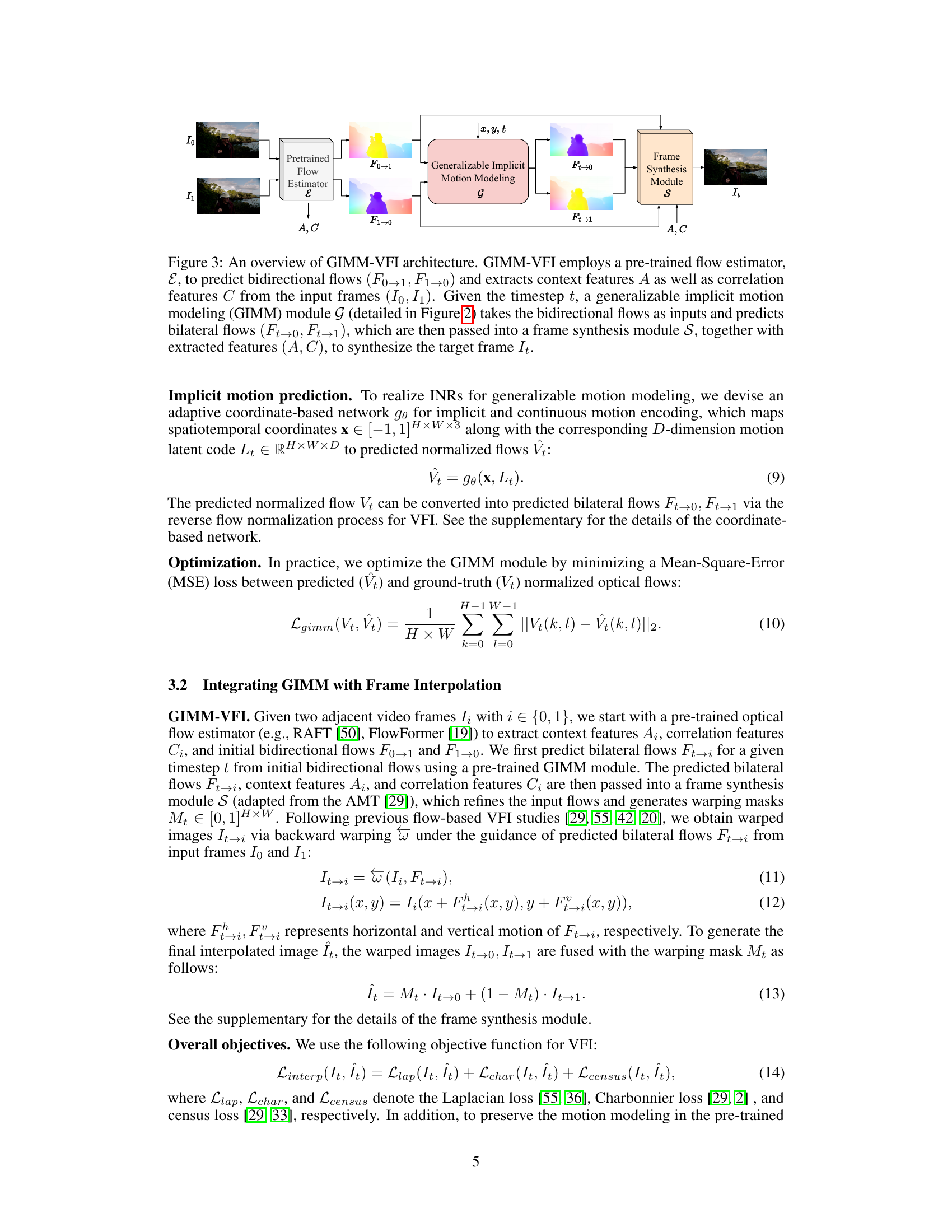
This paper introduces Generalizable Implicit Motion Modeling (GIMM), a new method for VFI that addresses these issues. GIMM uses a motion encoding pipeline to extract motion features from bidirectional flows, effectively capturing motion priors. Then, it implicitly predicts arbitrary-timestep optical flows using an adaptive coordinate-based neural network, achieving improved accuracy compared to prior art. The integration of GIMM into existing flow-based VFI frameworks is straightforward and leads to state-of-the-art performance on standard benchmarks.
Key Takeaways#
Why does it matter?#
This paper is important because it introduces a novel and effective approach to motion modeling for video frame interpolation, achieving state-of-the-art performance. It addresses limitations of existing methods by using a generalizable implicit motion modeling framework (GIMM) to accurately predict optical flow for arbitrary timesteps. This opens new avenues for research in video interpolation and related areas such as video compression and novel view synthesis. The GIMM method could significantly improve the quality of interpolated frames in various applications, and its generalizability makes it highly relevant to current research trends in implicit neural representation.
Visual Insights#

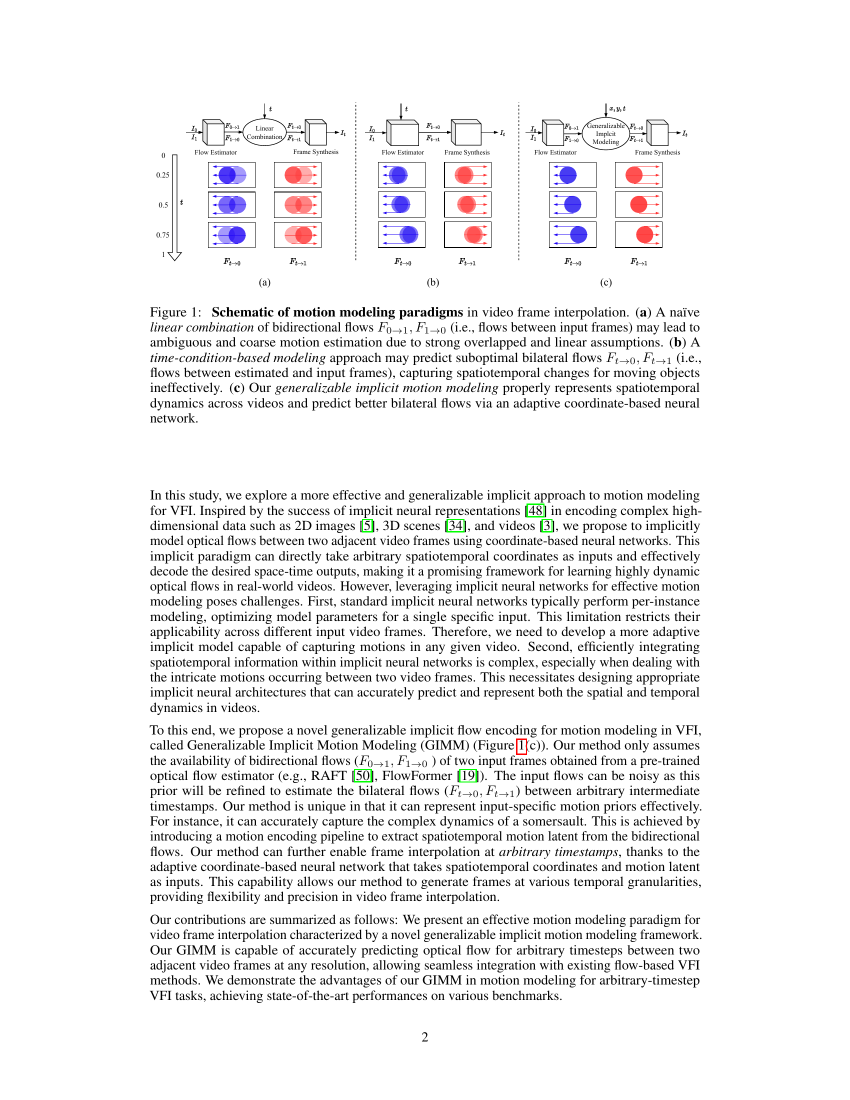
This figure compares three different motion modeling paradigms in video frame interpolation. (a) shows a naive linear combination of bidirectional flows, which is prone to errors due to strong overlapped and linear assumptions. (b) shows a time-conditioned approach that directly predicts bilateral flows for specific timestamps, but it lacks the ability to effectively model spatiotemporal dynamics. (c) introduces the proposed generalizable implicit motion modeling approach, which uses an adaptive coordinate-based neural network to model spatiotemporal dynamics more accurately and predict better bilateral flows.

This table compares different motion modeling methods (Linear, Forward Warp, End-to-End, BMBC, and GIMM) by evaluating their performance on three metrics: PSNRf (Peak Signal-to-Noise Ratio for optical flows), EPE (Endpoint Error for optical flows), and PSNRi (Peak Signal-to-Noise Ratio for interpolated images). The evaluation is performed on two datasets (Vimeo-Triplet-Flow and Vimeo-Septuplet-Flow) and a subset of SNU-FILM-arb, providing a comprehensive assessment of each method’s ability to model motion and its impact on video frame interpolation.
In-depth insights#
Implicit Motion#
Implicit motion modeling in video frame interpolation (VFI) represents a significant advancement. Instead of explicitly calculating or predicting motion vectors, implicit methods leverage neural networks to learn a mapping from spatiotemporal coordinates to the desired optical flow. This approach offers several advantages. Firstly, it avoids the limitations of explicit methods, such as those relying on linear combinations of bidirectional flows, which struggle with complex, real-world movements. Secondly, implicit modeling enables continuous interpolation, generating frames at arbitrary timesteps rather than being limited to discrete intervals. Thirdly, generalizability is enhanced as implicit models can be trained to capture motion dynamics across diverse video scenes. However, challenges remain, primarily regarding the computational cost of training and the potential for artifacts in cases of highly complex or occluded motion. Further research is needed to optimize implicit models for efficiency and robustness, particularly for high-resolution videos and scenes with extensive dynamic range.
GIMM-VFI Model#
The GIMM-VFI model represents a novel approach to video frame interpolation (VFI) by integrating a generalizable implicit motion modeling (GIMM) framework. GIMM excels at modeling complex spatiotemporal dynamics in videos, surpassing limitations of previous linear combination or direct prediction methods. By encoding motion latent from bidirectional flows, GIMM implicitly predicts flows for arbitrary timesteps, enabling accurate frame generation. Its key strength lies in the generalizability across various videos, avoiding per-instance optimization. Integration with existing flow-based VFI methods is straightforward, making GIMM-VFI a versatile and effective solution. The results suggest that GIMM-VFI significantly improves motion modeling and interpolation quality, achieving state-of-the-art performance on various benchmarks. However, the model’s reliance on a pre-trained flow estimator and its handling of highly complex motions remain points for potential future improvements.
Motion Encoding#
The concept of ‘Motion Encoding’ in video frame interpolation is crucial for effectively capturing and representing the dynamic movement in videos. A successful motion encoding strategy must robustly handle diverse motion patterns, including complex, non-linear movements and occlusions. Generalizability across various video types is essential, avoiding overfitting to specific video characteristics. The paper’s proposed method, likely involving a neural network architecture, aims to extract meaningful representations of motion from pre-trained flow estimators. This suggests that it focuses on learning latent features from the flow field to create a compact and informative representation. The method’s success hinges on its ability to effectively capture spatial-temporal dependencies, not just isolated motion vectors, which would allow for accurate flow prediction between arbitrary frames. The key innovation likely lies in how these latent features are generated and integrated into the overall interpolation process, enabling accurate prediction of intermediate frames. Finally, efficiency is vital, as real-time or near real-time performance is a common goal for video frame interpolation.
Ablation Studies#
Ablation studies systematically remove components of a model to assess their individual contributions. In the context of video frame interpolation, this could involve disabling parts of the motion modeling pipeline, such as the motion encoder or latent refiner, to evaluate their impact on overall performance. The key is to isolate the effect of each component, determining if it is essential and quantifying its importance. By comparing the performance of the full model to those with components removed, researchers can gain insights into model design and prioritize areas for further improvement. Results might reveal, for instance, that forward warping is crucial for accurately capturing complex temporal dynamics, or that the latent refiner significantly enhances the quality of motion estimation. Moreover, ablation studies reveal the relative importance of different design choices, enabling researchers to make informed decisions regarding model complexity and efficiency in future iterations. Ultimately, ablation studies offer an indispensable way to understand model architecture, improve performance and highlight promising research avenues.
Future Work#
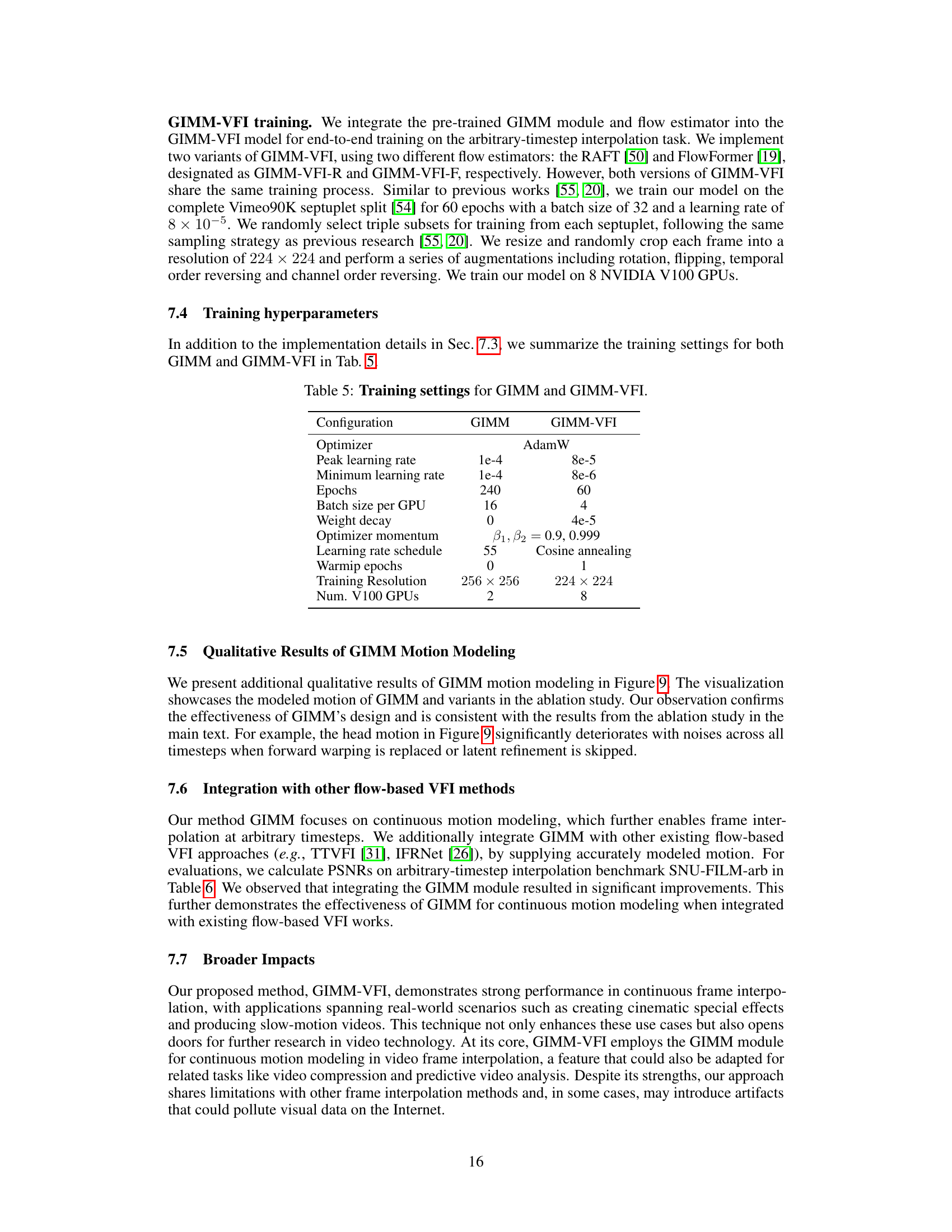
Future research directions stemming from this generalizable implicit motion modeling (GIMM) for video frame interpolation could explore several promising avenues. Extending GIMM to handle more complex scenarios such as significant occlusions, drastic illumination changes, and highly dynamic motions in videos would be beneficial. Improving the efficiency of GIMM by exploring more efficient network architectures or training strategies is also crucial for real-time applications. Investigating the applicability of GIMM to other video processing tasks beyond frame interpolation, such as video inpainting, super-resolution, or novel view synthesis, is a natural extension. Finally, a deeper investigation into the theoretical properties of GIMM, including its generalization capabilities and robustness to noise, is needed to provide a more comprehensive understanding of its capabilities and limitations. Addressing these areas would significantly advance the field of video processing and pave the way for more advanced and realistic video manipulation techniques.
More visual insights#
More on figures

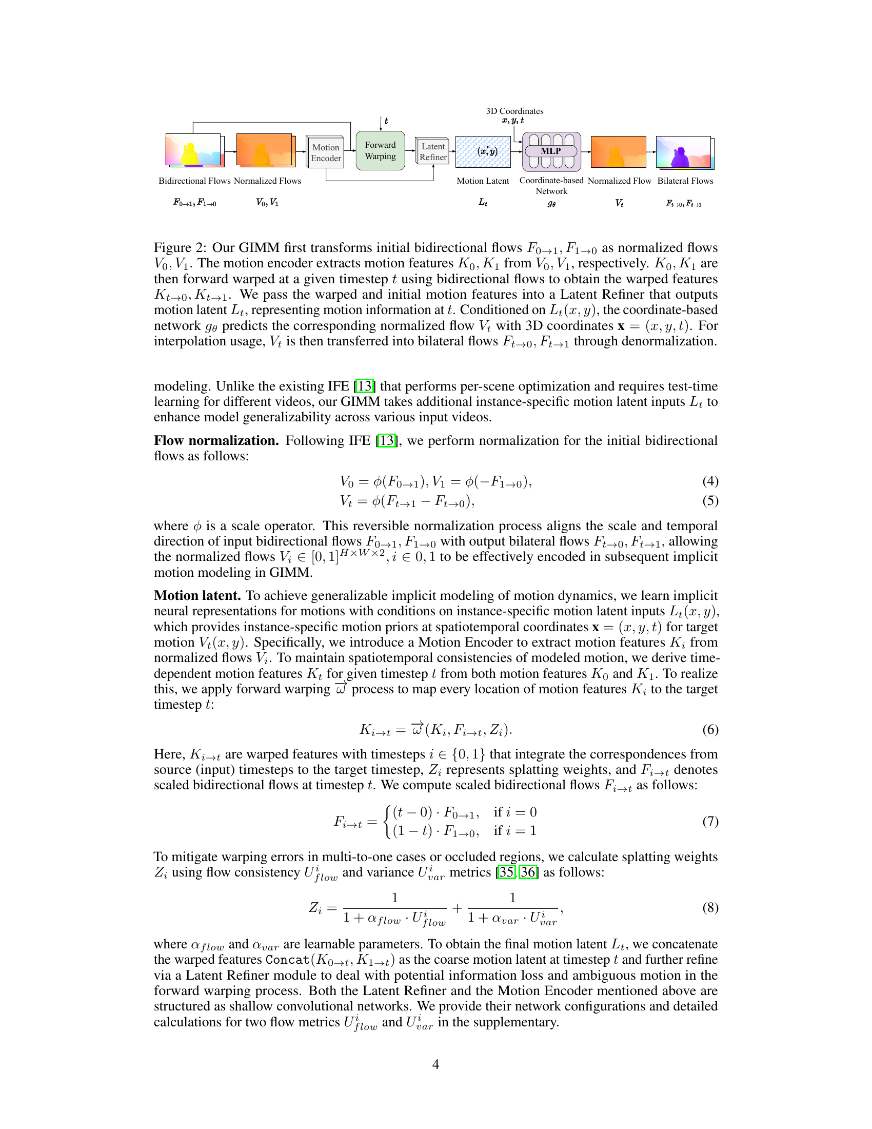
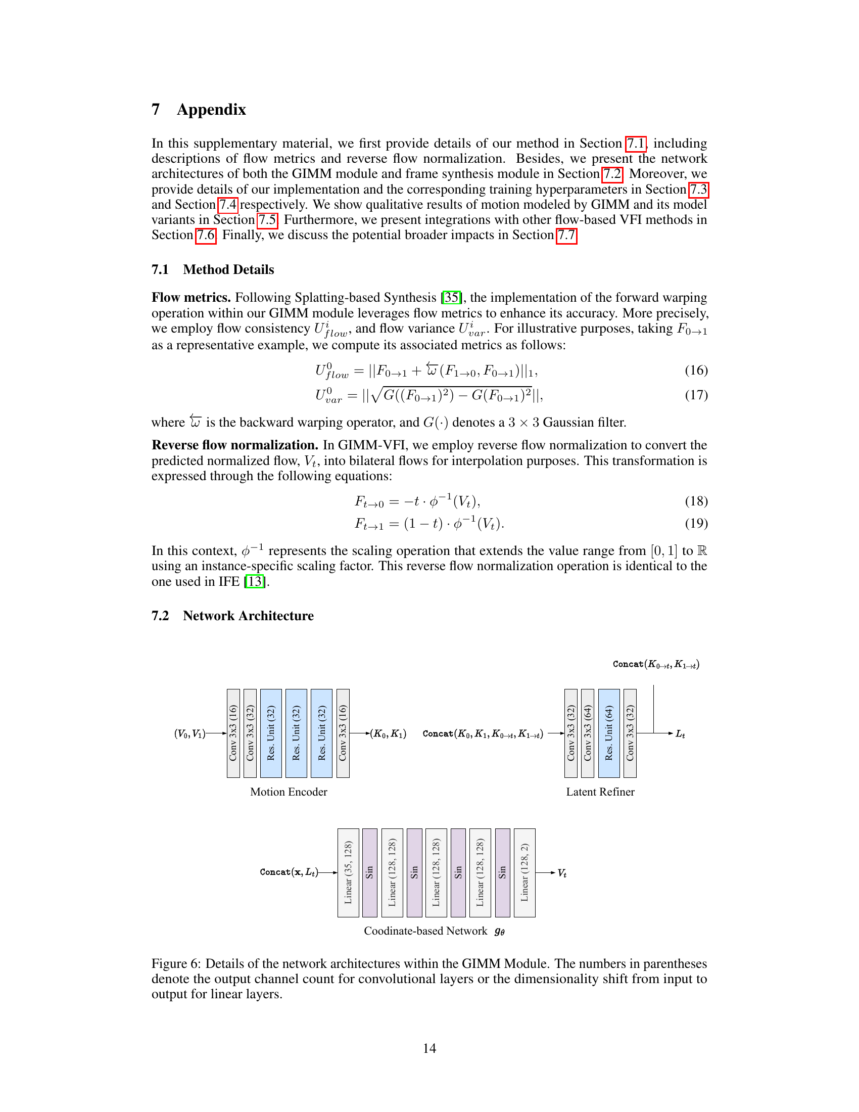
This figure illustrates the architecture of the Generalizable Implicit Motion Modeling (GIMM) module. It shows how bidirectional optical flows are normalized, encoded into motion features, and then used to generate implicit motion representations. These representations are then used by a coordinate-based network to predict normalized flows at arbitrary timesteps, which are finally denormalized to obtain bilateral flows.

This figure presents a qualitative comparison of various motion modeling methods’ performance on the SNU-FILM-arb-Hard dataset. The methods compared include Linear, Forward Warp, End-to-End, BMBC, and the proposed GIMM-VFI-R. Each method’s output is shown alongside the ground truth optical flow, illustrating the differences in motion prediction accuracy. The results displayed are for a specific timestep (t=0.75). The figure aims to visually demonstrate GIMM-VFI-R’s superior performance in accurately modeling complex motions.
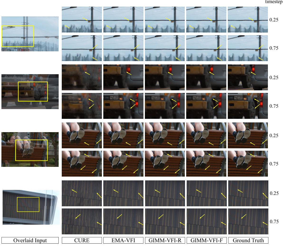
This figure compares the performance of different video frame interpolation methods on the XTest-2K benchmark at two different timesteps (0.25 and 0.75). The methods compared are CURE, EMA-VFI, GIMM-VFI-R, GIMM-VFI-F, and a ground truth. Each row shows a different video sequence, highlighting the interpolation results for various complex motions. The yellow arrows indicate specific areas where the proposed GIMM-VFI method demonstrates superior performance in handling challenging motion scenarios and preserving details.

This figure illustrates the architecture of the Generalizable Implicit Motion Modeling (GIMM) module. It shows how initial bidirectional flows are normalized, motion features are extracted and warped, and a latent motion representation is generated. This latent representation, along with spatiotemporal coordinates, is fed to a coordinate-based network to predict normalized flows, which are then denormalized to produce bilateral flows for video frame interpolation.
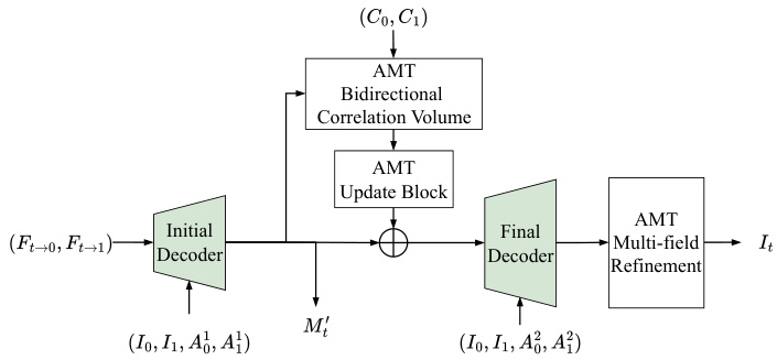
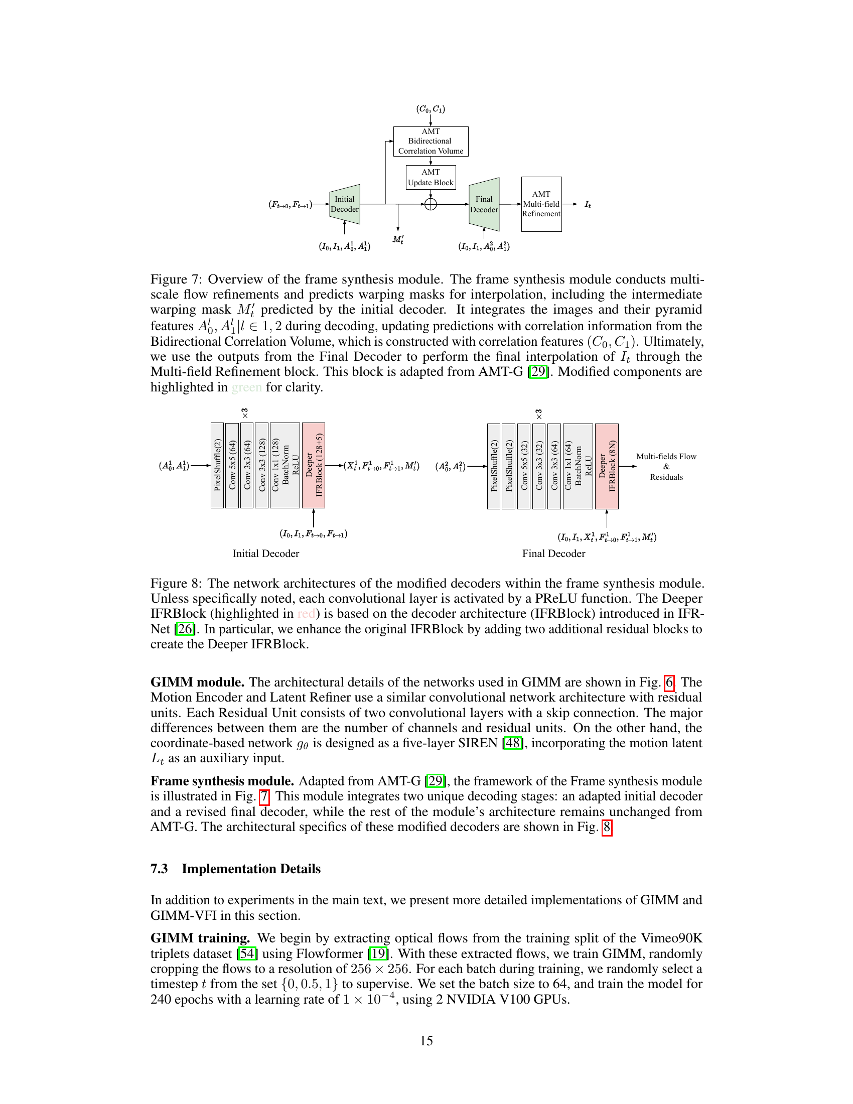
This figure shows the architecture of the frame synthesis module, which takes the predicted bilateral flows, context features, and correlation features as input to generate the final interpolated frame. It consists of an initial decoder, an update block, a final decoder, and a multi-field refinement block. The initial decoder predicts an intermediate warping mask, which is then refined by the update block and the final decoder. The multi-field refinement block combines the final warped images to generate the final interpolated frame. The module is based on AMT-G [29], with some modifications highlighted in green.

This figure details the network architectures of the modified decoders within the frame synthesis module. It highlights the use of a modified IFRBlock (Deeper IFRBlock), which is based on the IFRBlock from IFR-Net [26] but enhanced with two additional residual blocks. The figure shows the structures of both the Initial Decoder and the Final Decoder, showing the convolutional layers, activation functions (PReLU), and connections between different components within the decoder modules.

This figure provides a qualitative comparison of the GIMM model’s performance in 6X motion modeling on the Vimeo-septuplet-flow dataset. It compares the results of the full GIMM model against several ablation variants, each of which removes or modifies a specific component of the GIMM framework. These ablation studies investigate the effects of removing different architectural components such as the forward warping, the implicit model, latent refinement, and spatial coordinates, allowing for an assessment of their relative contributions to the model’s effectiveness.
More on tables

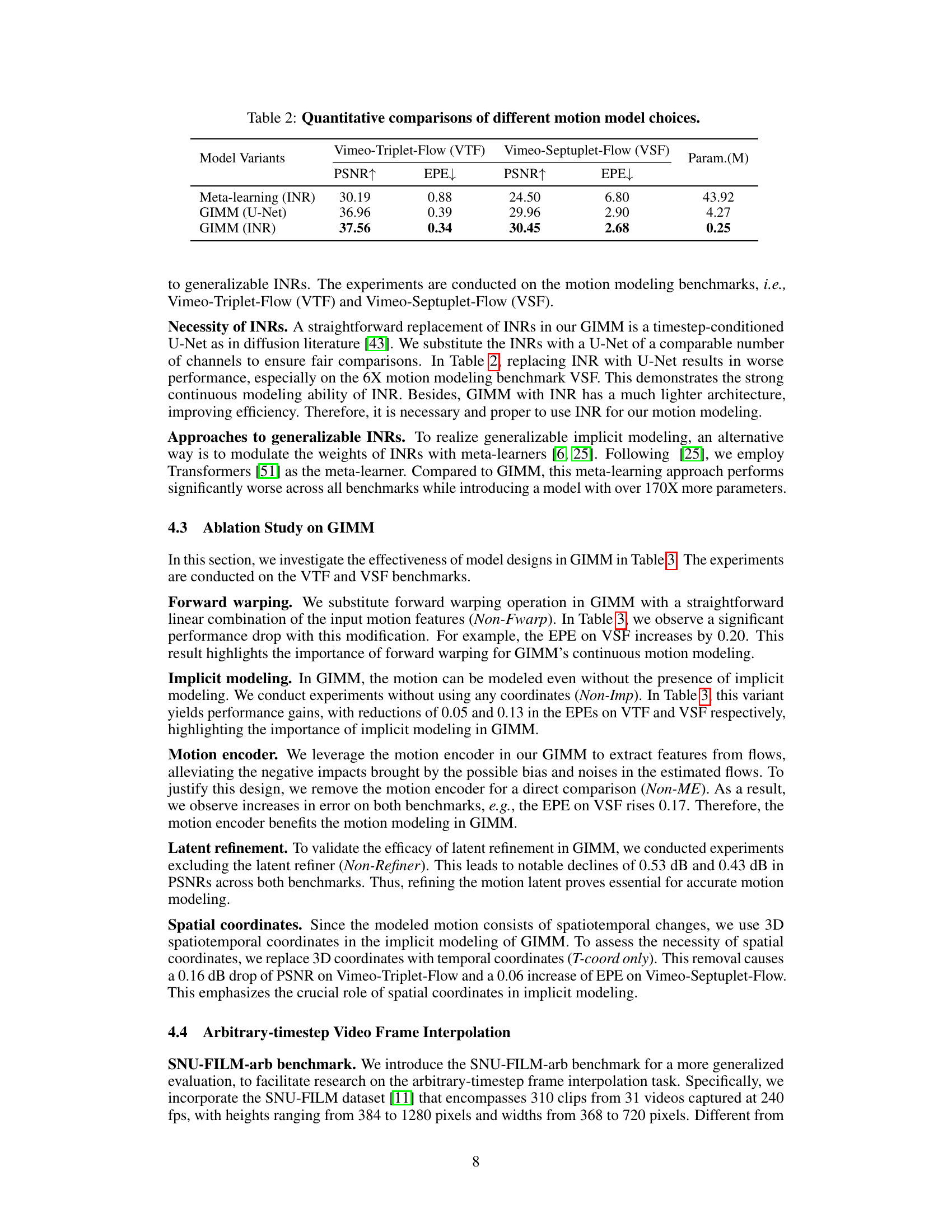
This table presents a quantitative comparison of different motion model choices on two video frame interpolation benchmarks: Vimeo-Triplet-Flow (VTF) and Vimeo-Septuplet-Flow (VSF). The metrics used for comparison are PSNR (higher is better) and EPE (lower is better), which evaluate the quality of the estimated motion. The models compared include a meta-learning approach using Implicit Neural Representations (INRs), a GIMM model using a U-Net architecture, and the proposed GIMM model using INRs. The table also shows the number of model parameters (in millions) for each model.
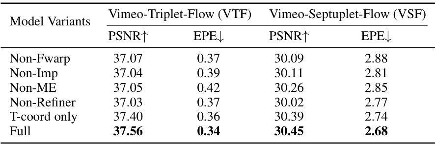
This table presents a quantitative comparison of different model variants of the proposed GIMM (Generalizable Implicit Motion Modeling) method. The variants are ablation studies exploring the impact of different design choices in the GIMM model on its motion modeling performance. Evaluated on two benchmarks, Vimeo-Triplet-Flow (VTF) and Vimeo-Septuplet-Flow (VSF), it assesses how modifications to components like forward warping, implicit modeling, the motion encoder, latent refinement, and the use of spatial coordinates influence the final PSNR (Peak Signal-to-Noise Ratio) and EPE (End-Point Error). The ‘Full’ row represents the complete, unmodified GIMM model.

This table compares different motion modeling methods (Linear, Forward Warp, End-to-End, BMBC, GIMM-VFI-R) by evaluating their performance using PSNR and EPE metrics on the Vimeo-Triplet-Flow (VTF) and Vimeo-Septuplet-Flow (VSF) datasets. It further shows the impact of these methods on the video frame interpolation task by reporting the PSNR of the interpolated images on the ‘hard’ split of the SNU-FILM-arb dataset. PSNRf represents PSNR for optical flows, and PSNRi represents PSNR for interpolated images.
This table compares different motion modeling methods for video frame interpolation. It shows the Peak Signal-to-Noise Ratio (PSNR) and Endpoint Error (EPE) metrics for the modeled motion on the Vimeo-Triplet-Flow (VTF) and Vimeo-Septuplet-Flow (VSF) datasets. It also includes the PSNR for the interpolated images on the ‘hard’ split of the SNU-FILM-arb dataset to show the impact of motion modeling on interpolation performance. PSNRf represents PSNR for optical flows, and PSNRi represents PSNR for interpolated images.

This table compares different motion modeling methods (Linear, Forward Warp, End-to-End, BMBC, and GIMM) by evaluating their performance on three different metrics: PSNRf (peak signal-to-noise ratio for optical flows), EPE (endpoint error for optical flows), and PSNRi (peak signal-to-noise ratio for interpolated images). The evaluation is performed on two datasets, Vimeo-Triplet-Flow and Vimeo-Septuplet-Flow, to assess motion quality, and on the ‘hard’ split of the SNU-FILM-arb dataset to assess the impact of motion modeling on the interpolation task.
Full paper#

