↗ OpenReview ↗ NeurIPS Homepage ↗ Chat
TL;DR#
Many existing methods for learning time-series representations rely on the assumption that the original temporal order is optimal for learning. However, this may not always be true, particularly for complex real-world time series where dependencies may exist between non-adjacent sections. This paper explores the impact of alternative time series arrangements on representation learning by introducing a novel plug-and-play layer called Segment, Shuffle, and Stitch (S3). The existing approaches may struggle to capture these long-range dependencies, hindering effective representation learning.
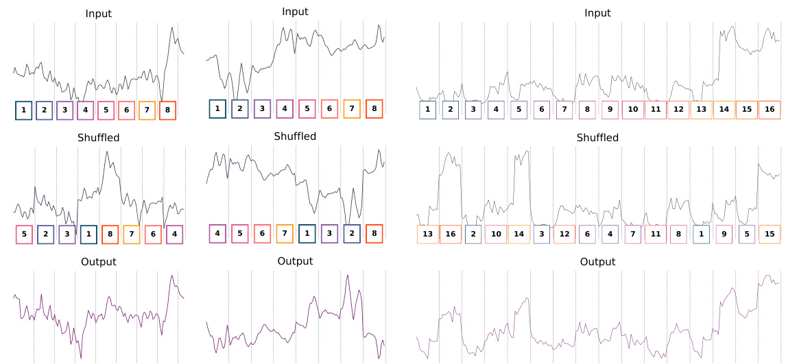
The proposed S3 layer addresses this by creating non-overlapping segments of the original time series and then shuffling those segments in a learned manner determined by the downstream task. This shuffled sequence, combined with the original sequence via a learned weighted sum, is then passed to the rest of the model. The results on various benchmark datasets (including classification, forecasting and anomaly detection) show significant improvements in model performance compared to various state-of-the-art baselines, demonstrating the effectiveness of the approach. Furthermore, it is shown that S3 makes training more stable, with a smoother training loss curve.
Key Takeaways#
Why does it matter?#
This paper is crucial for researchers working with time-series data because it introduces a novel and efficient layer (S3) that significantly improves the performance of existing time-series models across various tasks. The modularity and ease of integration of S3 make it highly adaptable to diverse neural architectures, broadening its applicability and potential impact on various research fields. This work addresses limitations of current deep learning approaches for time series, particularly their struggles with capturing long-range dependencies in data, thus, paving the way for improved methodologies across various time-series data applications.
Visual Insights#

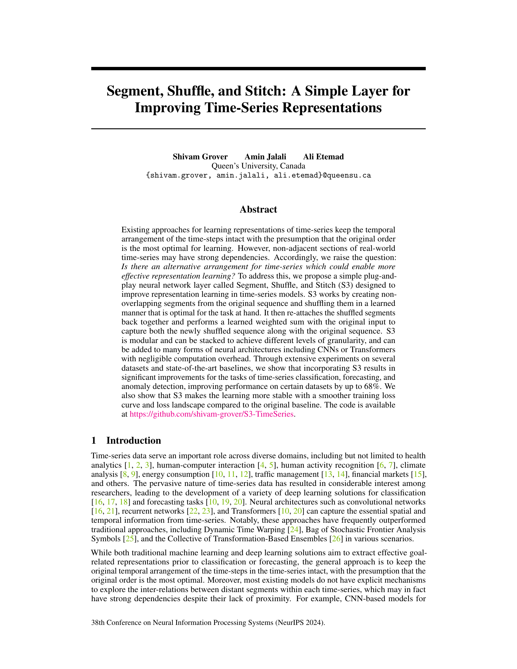
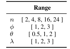
This figure shows how multiple S3 layers can be stacked to achieve different levels of granularity in time series processing. Each S3 layer consists of three steps: segment, shuffle, and stitch. The segment step divides the input time series into non-overlapping segments. The shuffle step rearranges these segments in a learned manner that is optimal for the task at hand. The stitch step re-attaches the shuffled segments back together. The hyperparameters n, Φ, and θ control the number of segments, the number of S3 layers, and the multiplier for the number of segments in subsequent layers, respectively. By stacking multiple S3 layers, the model can perform shuffling at different granularity levels, improving the ability of the model to capture long-range dependencies in the time series.
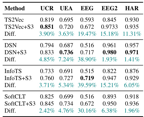
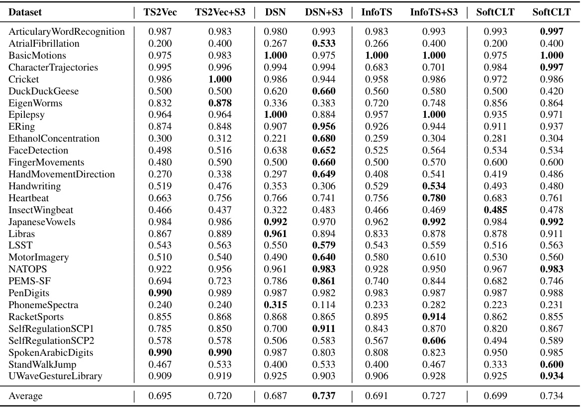
This table presents the classification accuracy results of four different state-of-the-art time-series classification methods, namely TS2Vec, DSN, InfoTS, and SoftCLT. For each method, the accuracy is shown both without and with the addition of the proposed S3 layer. The ‘Diff.’ column shows the percentage improvement in accuracy achieved by adding the S3 layer. The results are averaged across five different datasets (UCR, UEA, EEG, EEG2, and HAR) commonly used in the time-series classification literature.
In-depth insights#
S3 Layer Design#
The S3 layer, standing for Segment, Shuffle, and Stitch, is designed as a modular and flexible layer for enhancing time-series representation learning. Its core functionality involves three steps: first, segmenting the input time-series into non-overlapping segments; second, shuffling these segments according to a learned permutation, controlled by learnable parameters, aiming to capture non-adjacent dependencies effectively. Finally, the shuffled segments are stitched back together. A weighted sum with the original sequence is performed to integrate both shuffled and original information. The modularity of S3 allows for stacking multiple layers with different segment granularities, increasing the capacity to capture long-range temporal relationships. Learned shuffling parameters adapt to the specific task and backbone model, enabling goal-centric optimization. The design is computationally efficient, with negligible overhead and few hyperparameters.
Shuffle Mechanism#
The effectiveness of a time-series model hinges on its ability to capture inherent temporal dependencies. A novel approach, the ‘Shuffle Mechanism,’ addresses this by introducing a learnable permutation of time-series segments. Instead of relying solely on the original temporal order, this method dynamically rearranges segments in a way that’s optimal for the target task (classification, forecasting, etc.). This is achieved through a learned shuffling parameter vector, which learns the optimal arrangement during training. The key innovation lies in the differentiability of the shuffling process, enabling seamless integration into standard neural network architectures via gradient descent. This avoids discrete sorting operations that would disrupt backpropagation, facilitating more effective representation learning and model training. The method’s modularity allows it to be stacked, creating higher levels of granularity and complexity in the shuffling. Furthermore, incorporating a weighted sum with the original time-series sequence helps preserve important temporal features. This combined strategy ensures that the model benefits from both the original order and a potentially more informative arrangement, thereby enhancing its overall performance and stability.
Empirical Gains#
An ‘Empirical Gains’ section in a research paper would detail the quantitative improvements achieved by the proposed method. It would go beyond simply stating performance metrics; a strong section would carefully compare the results to established baselines using statistically sound methods, highlighting the magnitude and significance of the gains. Crucially, it would address potential confounding factors, such as variations in datasets, experimental setups, or hyperparameter choices, ensuring that the reported gains are not artifacts of these factors. The analysis should explain why the improvements were obtained, potentially linking them to specific design choices or theoretical properties of the proposed method. Furthermore, the section should visualize results, using charts and graphs to clearly and compellingly demonstrate the advantages. Finally, discussion of any unexpected or counterintuitive results should be included, strengthening the analysis and its conclusions.
Ablation Study#
An ablation study systematically removes components of a model to assess their individual contributions. In the context of the provided research paper, an ablation study on the proposed ‘Segment, Shuffle, and Stitch’ (S3) layer would involve selectively disabling parts of the S3 process, such as the segmentation, shuffling, or stitching steps, to gauge their impact on performance. By comparing the performance of the full S3 model against these ablated versions, the researchers can determine the relative importance of each component. For example, removing the shuffling step would test whether the learned reordering of segments is crucial to performance improvements, while disabling the stitching step would reveal whether the integration of shuffled and original sequences is necessary. These experiments would provide strong evidence supporting the claims of the paper by quantitatively isolating the contribution of each component to the overall performance gains. Furthermore, the ablation study helps to identify any potential redundancy or unnecessary complexity in the S3 design, providing insights for future model optimization and refinement. The results of the ablation study are critical to establishing the integrity and effectiveness of the proposed S3 layer as a modular and versatile component within various time-series models. A comprehensive ablation study strengthens the paper’s overall methodology and credibility.
Future Work#
The paper’s ‘Future Work’ section would greatly benefit from exploring the applicability of the S3 layer to diverse time-series modalities beyond the tested datasets. Investigating its performance on video data, sensor streams, or other high-dimensional time-series would significantly broaden its impact. Furthermore, a detailed investigation into the interplay between the S3 layer’s hyperparameters and the characteristics of different datasets is crucial. Developing a more principled and data-driven approach to hyperparameter selection would enhance the layer’s usability and performance predictability. A natural extension is to explore the integration of S3 with other advanced techniques, like attention mechanisms, transformers, or graph neural networks, to further boost performance and discover synergistic benefits. Additionally, a thorough comparative study against other recent approaches to time-series representation learning is necessary to definitively establish S3’s advantages and limitations. Finally, a focus on theoretical analysis to understand why and when S3 works best could lead to a more profound understanding and potential improvements to the algorithm.
More visual insights#
More on figures

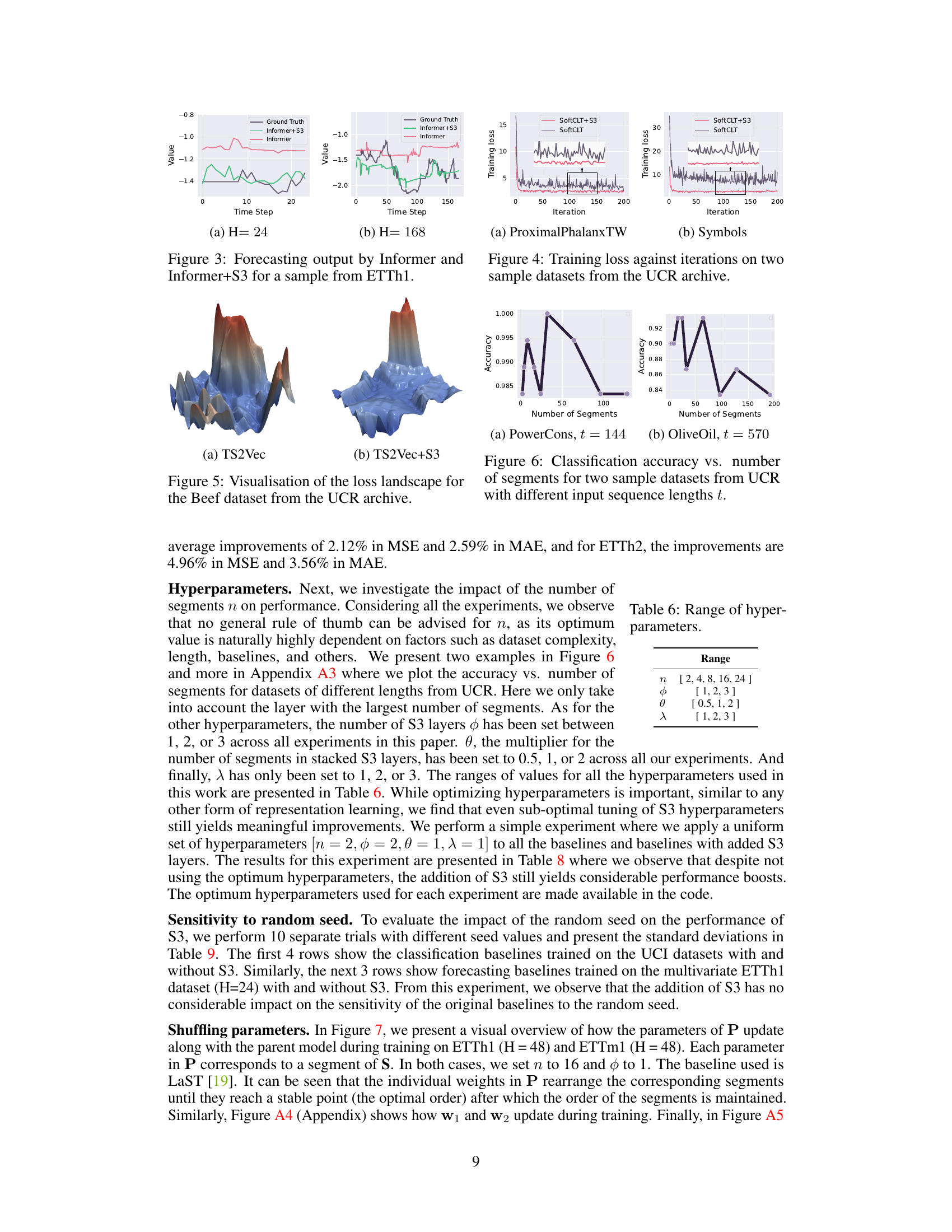
This figure shows the forecasting results of the Informer model with and without the proposed S3 layer. Two different forecast horizons (H=24 and H=168) are presented, comparing the model’s predictions against the ground truth. The plots visually demonstrate that incorporating the S3 layer leads to improved forecasting accuracy for both forecast horizons. The model with S3 more accurately reflects the trends and patterns in the ground truth.

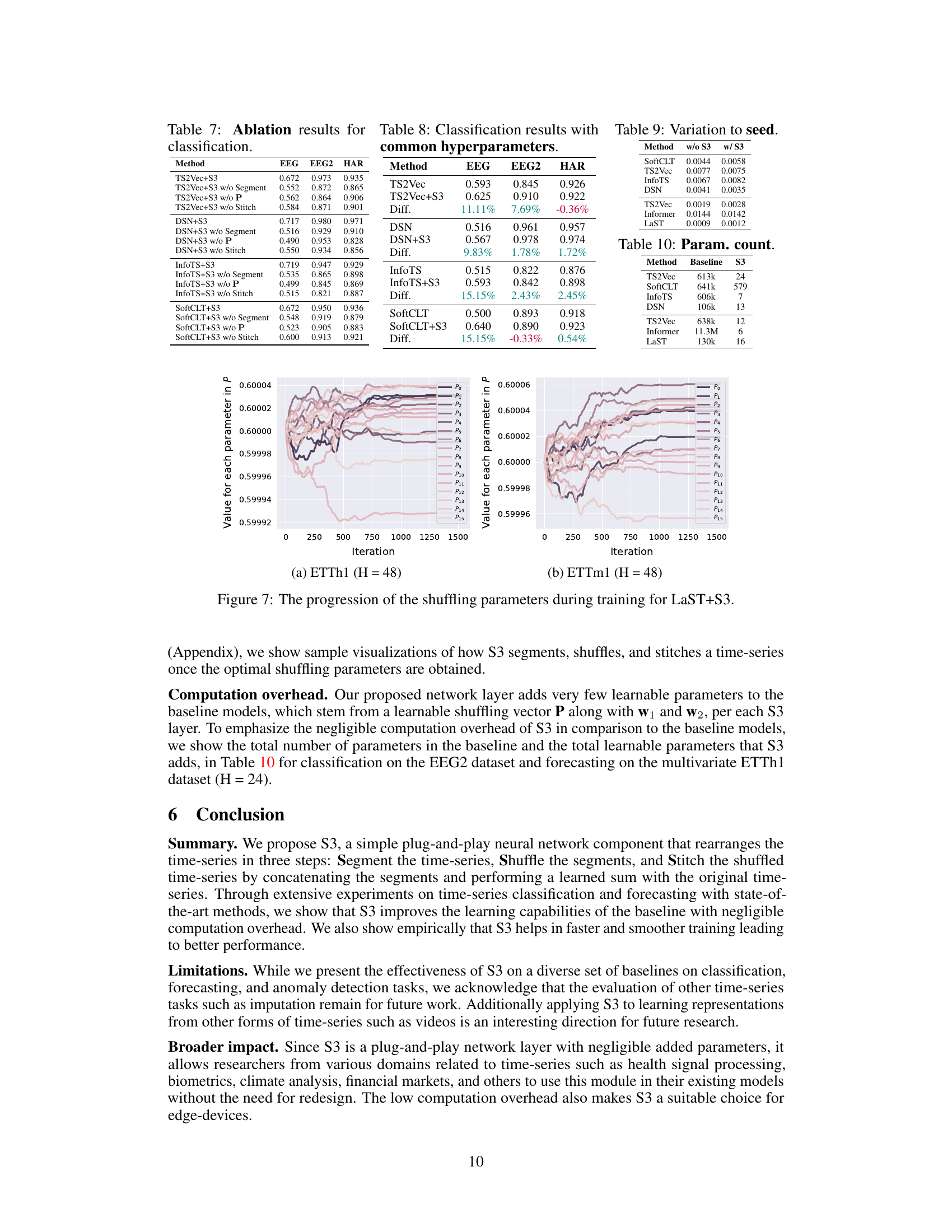
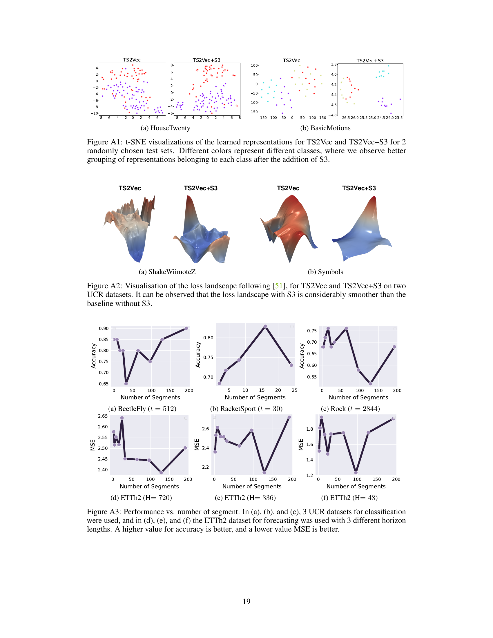
This figure visualizes the loss landscape for TS2Vec with and without the proposed S3 layer on two datasets from the UCR archive. The loss landscape is a representation of the loss function across different parameter settings. A smoother loss landscape typically indicates more stable training. This figure demonstrates that integrating S3 leads to a significantly smoother loss landscape compared to the baseline, implying more stable training dynamics and potentially improved generalization.
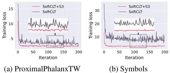
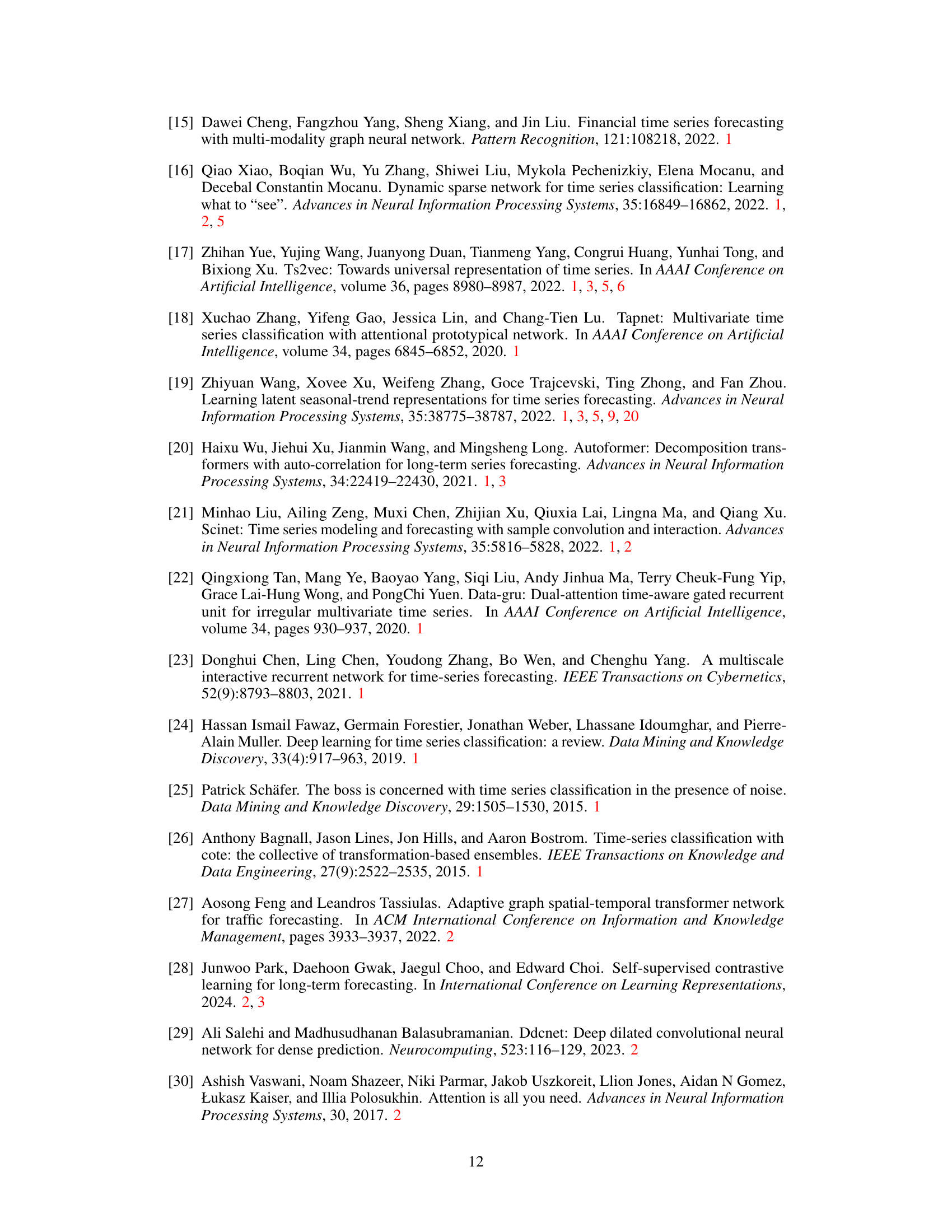
The figure shows the training loss curves for two datasets from the UCR archive (ProximalPhalanxTW and Symbols) with and without the proposed S3 layer. It demonstrates that the S3 layer leads to faster convergence and smoother training loss curves compared to the baselines.
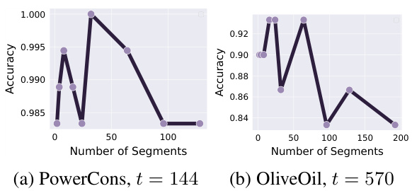
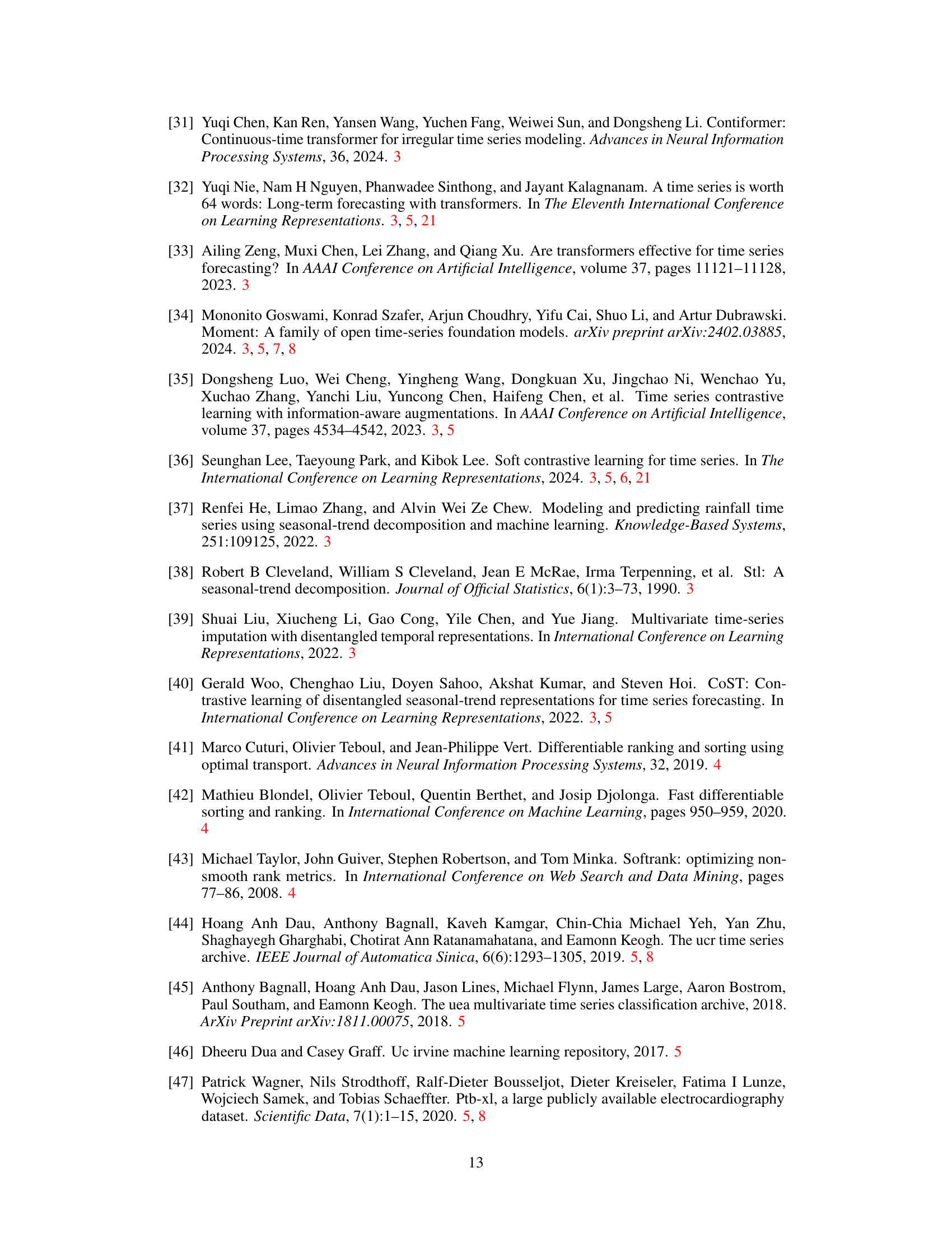
This figure shows the impact of the number of segments on the performance of the proposed S3 layer for both classification and forecasting tasks. Three UCR datasets (Beetlefly, RacketSport, and Rock) are used for classification, while the ETTh2 dataset is used for forecasting with three different horizon lengths (720, 336, and 48). The results demonstrate that an optimal number of segments exists for each dataset and task, highlighting the importance of this hyperparameter in achieving the best performance.

This figure illustrates the modular design of the S3 layer, showing how multiple S3 layers can be stacked to achieve different levels of granularity in time-series shuffling. Each S3 layer consists of three steps: Segment, Shuffle, and Stitch. The hyperparameters n, , and control the number of segments, the number of layers, and the multiplier for the number of segments in subsequent layers, respectively. The figure shows an example with 2 segments per layer and 3 layers stacked, demonstrating how the time series data is progressively shuffled and processed.

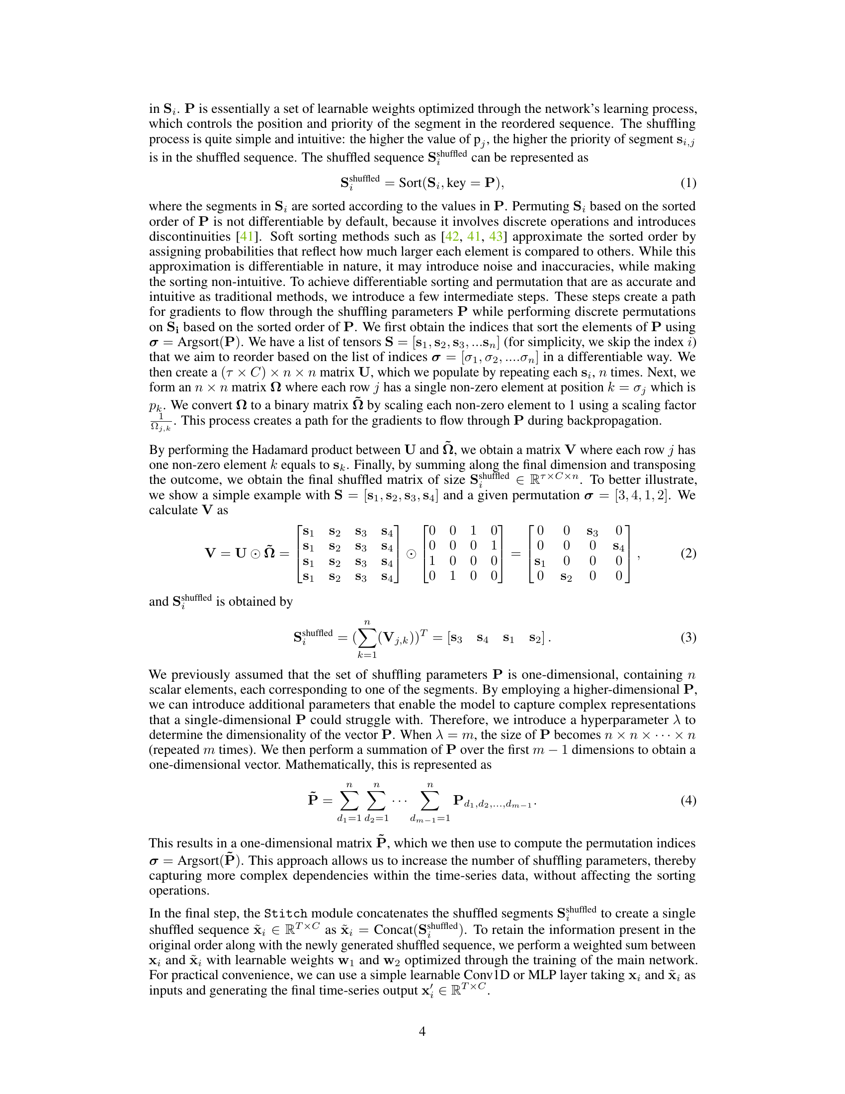
This figure shows the t-distributed Stochastic Neighbor Embedding (t-SNE) visualizations of the learned representations by TS2Vec with and without the S3 layer. Two randomly selected test sets from the UCR dataset are used. Each point represents a data sample, and the color represents its class label. The plots demonstrate that after adding the S3 layer, the representations of different classes are more separable in the t-SNE space, indicating improved class separability.

This figure shows t-SNE visualizations of the learned representations using TS2Vec with and without the proposed S3 layer. Two different UCR datasets are used, and each plot shows the resulting clusters of data points in 2-dimensional space, with different colors representing different classes. The addition of the S3 layer results in a clearer separation of the classes, indicating improved representation learning and better class separability.

This figure visualizes the impact of the number of segments (n) on the performance of the proposed S3 layer. It shows the accuracy and MSE for three classification datasets (BeetleFly, RacketSport, Rock) and three forecasting datasets (ETTh2 with different horizons) using different numbers of segments. This demonstrates the effect of segmenting the time series with varying granularity on the model’s performance. The optimal number of segments differs depending on the dataset and task, highlighting the adaptive nature of the S3 layer.
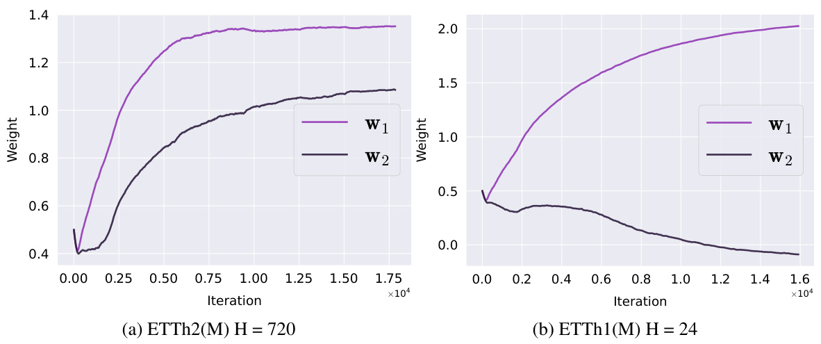
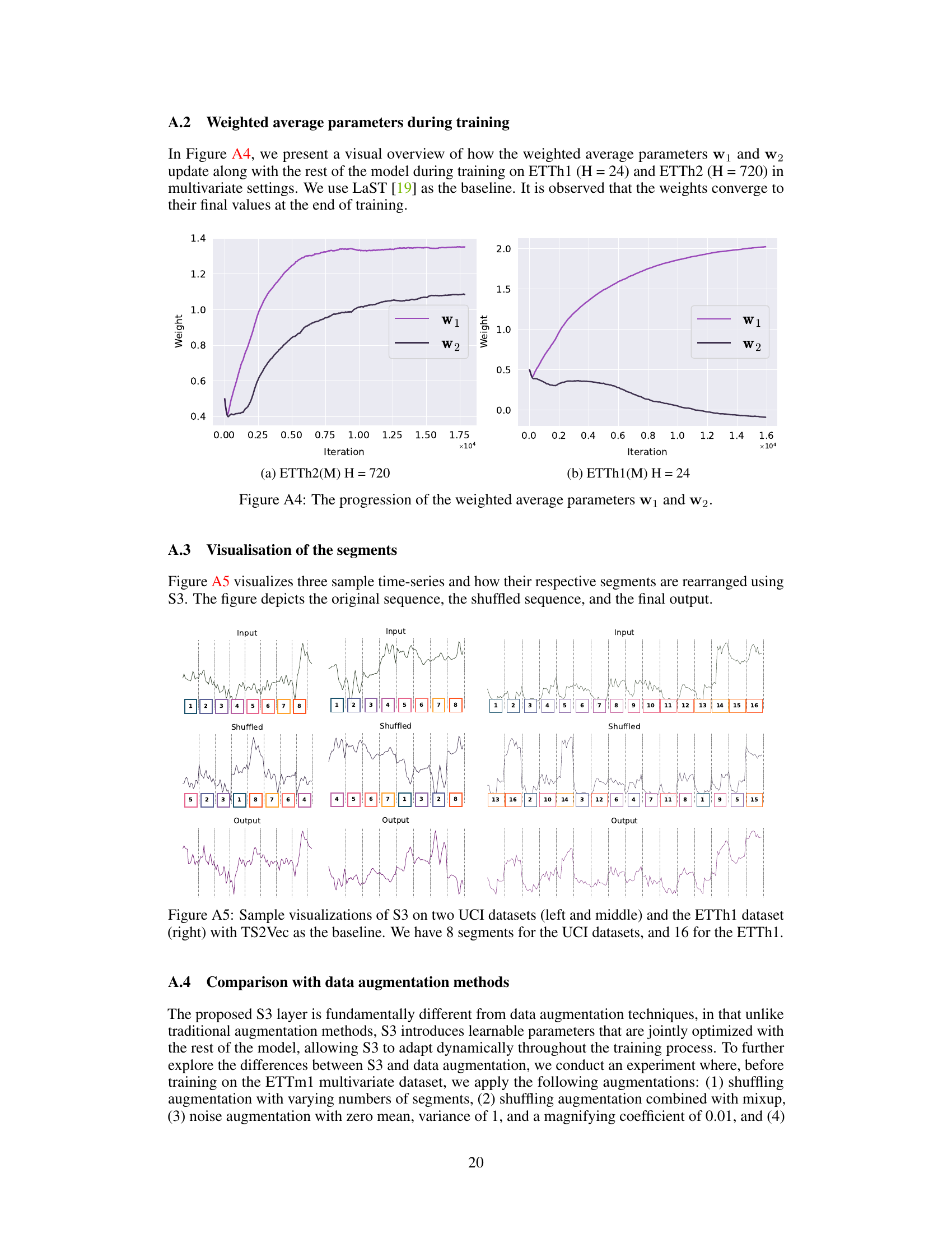
This figure visualizes how the weighted average parameters w1 and w2 change during the training process for two different multivariate forecasting datasets: ETTh2(M) with a horizon (H) of 720 and ETTh1(M) with a horizon of 24. The plots show the values of w1 and w2 over the training iterations, illustrating their convergence towards final values.
This figure shows how multiple S3 layers can be stacked in a neural network. Each S3 layer consists of three operations: segment, shuffle, and stitch. The hyperparameters n, φ, and θ control the number of segments, the number of layers, and the multiplier for the number of segments in subsequent layers, respectively. The figure shows an example with n=2, φ=3, and θ=2, resulting in three S3 layers, each with a different number of segments.

This figure shows the relationship between the size of the LSST dataset and the performance improvement achieved by incorporating the S3 layer. Different subsets of the LSST dataset were created by randomly sampling varying amounts of data (ranging from 20% to 99%), and the SoftCLT model was trained with and without the S3 layer on each of these subsets. The plot shows the average improvement in performance (as measured by the percentage difference in MSE) for each dataset size, averaged over three independent runs. The results suggest that there is no clear trend in the performance improvement as a function of dataset size, indicating that the S3 layer’s benefits are consistent regardless of dataset size.
More on tables
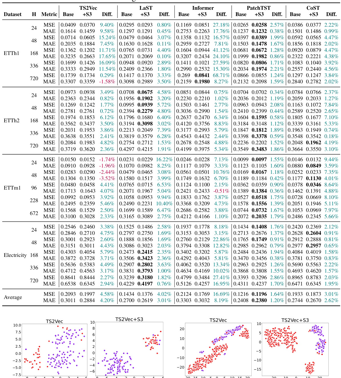
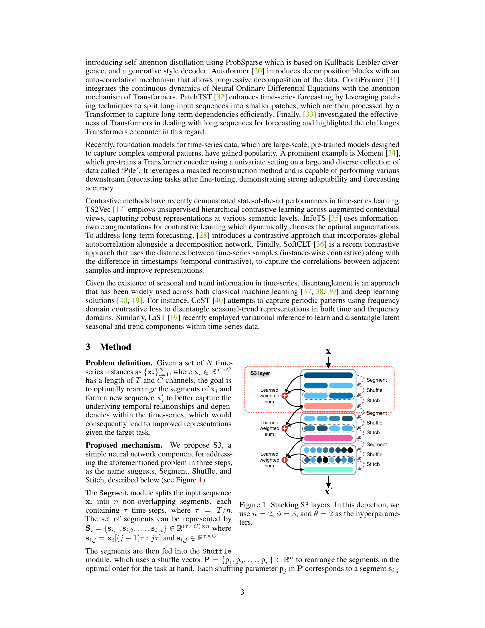
This table presents the results of univariate forecasting experiments conducted on various datasets using different forecasting horizons (H). It compares the performance of several state-of-the-art baseline models (TS2Vec, LaST, Informer, PatchTST, and CoST) against the same models enhanced with the proposed S3 layer. For each dataset and horizon, the table shows the Mean Squared Error (MSE) and Mean Absolute Error (MAE) for each baseline model and its S3-enhanced counterpart, along with the percentage difference in performance between the two. This allows for a quantitative assessment of the improvement offered by the S3 layer in univariate time-series forecasting tasks.

This table presents the results of univariate forecasting experiments conducted on various datasets and horizons (H) using different state-of-the-art baseline models. For each dataset and horizon, the Mean Squared Error (MSE) and Mean Absolute Error (MAE) are reported for both the original baseline model and the same model with the proposed S3 layer integrated. The ‘Diff.’ column shows the percentage difference in MSE and MAE between the baseline and baseline+S3 models, indicating the improvement achieved by incorporating the S3 layer.

This table presents the results for anomaly detection on Yahoo and KPI datasets. The anomaly score is computed as the L1 distance between two encoded representations derived from masked and unmasked inputs, following the methodology described in previous studies. The table shows the F1 score, precision, and recall for both datasets for the models TS2Vec, TS2Vec with the proposed S3 layer, SoftCLT, and SoftCLT with the S3 layer.
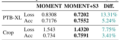
This table compares the performance of the pre-trained MOMENT model with and without the proposed S3 layer on two datasets: PTB-XL and Crop. For each dataset, it reports the loss and accuracy achieved by both models. The ‘Diff.’ column shows the percentage difference in loss and accuracy between the MOMENT+S3 model and the baseline MOMENT model. Positive values in the ‘Diff.’ column indicate that the MOMENT+S3 model outperformed the baseline model. This table demonstrates the effectiveness of the S3 layer when integrated into a pre-trained foundation model.
This table compares the classification accuracy of different models (TS2Vec, DSN, InfoTS, SoftCLT) with and without the proposed S3 layer across various datasets (UCR, UEA, EEG, EEG2, HAR). The ‘Diff.’ column shows the percentage improvement in accuracy achieved by adding the S3 layer. The results demonstrate the effectiveness of the S3 layer in enhancing the performance of different classification models and across various datasets.

This table presents the classification accuracy results for various state-of-the-art baseline models on several benchmark datasets, both with and without the integration of the proposed S3 layer. The ‘Diff.’ column indicates the percentage improvement achieved by adding the S3 layer. This allows for easy comparison and highlights the effectiveness of S3 in enhancing the classification performance of different models.

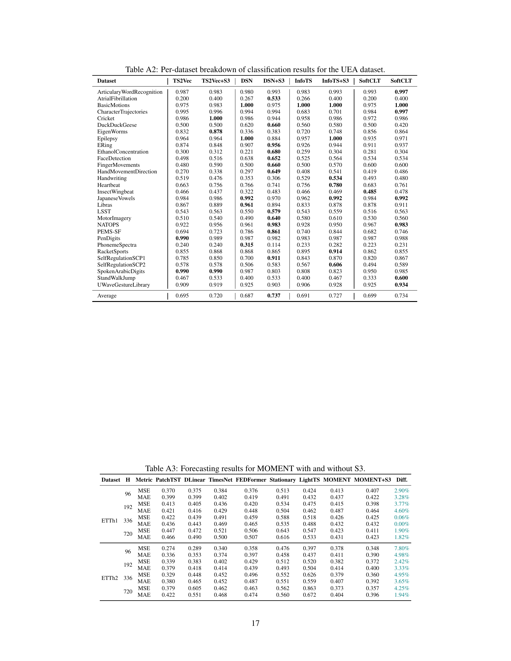
This table presents the classification accuracy results of different models on various datasets. It compares the performance of several state-of-the-art time-series classification models (TS2Vec, DSN, InfoTS, SoftCLT) with and without the proposed S3 layer. The ‘Diff.’ column shows the percentage improvement in accuracy achieved by adding the S3 layer to each baseline model. The results demonstrate improvements across all baselines and datasets, highlighting the effectiveness of the S3 layer in enhancing time-series representation learning for classification tasks.
This table presents a comprehensive overview of the results for univariate forecasting on different datasets and horizons (H), with and without the incorporation of S3. It shows the Mean Squared Error (MSE) and Mean Absolute Error (MAE) for various forecasting horizons (H) and different datasets. The ‘Diff.’ column indicates the percentage improvement achieved by incorporating S3 into each baseline model. The table allows for a direct comparison of the performance of different state-of-the-art models with and without the proposed S3 layer, providing evidence of S3’s effectiveness in enhancing time-series forecasting accuracy.
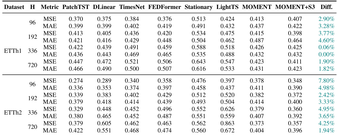
This table presents the results of univariate forecasting experiments conducted on various datasets and horizons (H). It compares the performance of several state-of-the-art baseline forecasting models (TS2Vec, LaST, Informer, PatchTST, and CoST) with and without the addition of the proposed S3 layer. For each model and dataset, the Mean Squared Error (MSE) and Mean Absolute Error (MAE) are reported, along with the percentage difference in these metrics resulting from the inclusion of S3. Positive percentage differences indicate improvements in performance (lower MSE and MAE are better).

This table presents the classification accuracy results on several datasets (UCR, UEA, EEG, EEG2, and HAR) for five different baselines (TS2Vec, DSN, InfoTS, SoftCLT) with and without the proposed S3 layer. The ‘Diff.’ column shows the percentage improvement in accuracy achieved by adding the S3 layer to each baseline model. The results highlight the consistent improvement in classification performance across various datasets and baselines when incorporating the S3 layer.
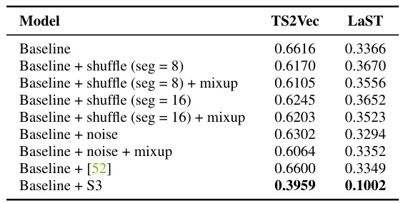
This table compares the performance of the proposed S3 layer against various data augmentation methods on the ETTm1 multivariate time series forecasting dataset. It shows that S3 significantly outperforms the other methods in terms of Mean Squared Error (MSE). The results demonstrate S3’s effectiveness in improving time series representation learning compared to traditional augmentation techniques.

This table presents the results of univariate forecasting experiments conducted on various datasets using different baseline models, both with and without the integration of the proposed S3 layer. The table includes metrics such as MSE and MAE for different forecast horizons (H). It highlights the improvement achieved by incorporating S3 into each baseline model, showing percentage difference in MSE and MAE values.
Full paper#
