↗ OpenReview ↗ NeurIPS Homepage ↗ Chat
TL;DR#
Gröbner basis computation is a core problem in computational algebra, known for its high computational complexity. Existing mathematical algorithms are often computationally intractable for large-scale polynomial systems. This paper explores a novel approach using machine learning to address this challenge. The core issue is the lack of efficient methods to generate sufficient training data (non-Gröbner set, Gröbner basis pairs) for the machine learning model. This necessitates the creation of new algebraic solutions for efficient data generation, a significant hurdle for previous attempts at using machine learning in this context.
This research proposes a learning-based method to compute Gröbner bases using Transformers, overcoming the data generation challenge. It introduces efficient algorithms for generating random Gröbner bases and transforming them into non-Gröbner forms (backward Gröbner problem). The study also employs a novel hybrid input embedding technique to represent polynomial coefficients effectively. Experiments demonstrate that the proposed dataset generation method is far more efficient than naive approaches and that computing Gröbner bases is indeed learnable within a specific class of polynomial systems, showing the potential of AI in tackling complex mathematical problems.
Key Takeaways#
Why does it matter?#
This paper is crucial because it tackles the computationally expensive problem of Gröbner basis computation, a fundamental task in computational algebra. By demonstrating the learnability of this NP-hard problem using Transformers, it opens new avenues for efficient polynomial system solving and offers insights into the underlying patterns of Gröbner bases. The novel algebraic problems addressed and the efficient dataset generation methods contribute significantly to the field, enabling future research in large-scale polynomial system analysis.
Visual Insights#

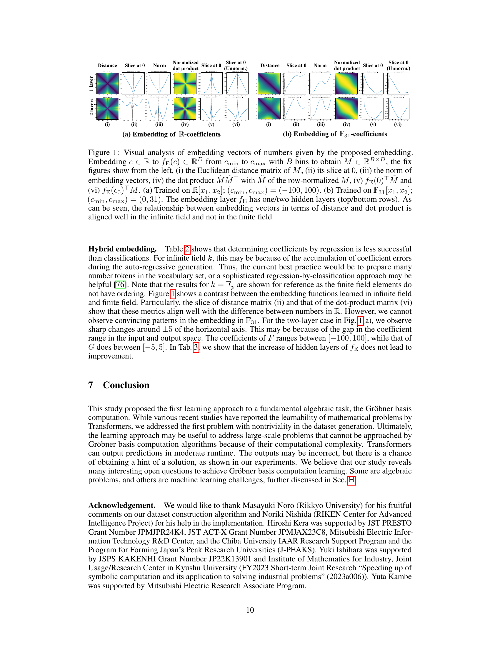
This figure visualizes the embedding vectors of numbers generated by the proposed hybrid embedding method. It compares the embeddings of real numbers (R) and finite field numbers (F31). The plots show Euclidean distance matrices, slices of these matrices, norms of embedding vectors, dot products of normalized embeddings, and dot products with specific embedding vectors (fE(0) and fE(c0)). The results highlight that the continuous embedding scheme better captures the relationships between numbers in the infinite field (R) compared to the finite field (F31).

This table compares the runtime of forward and backward generation methods for creating datasets of Gröbner bases. The forward method uses three different algorithms from SageMath, while the backward method is the one proposed by the authors. The table shows runtime for datasets with varying numbers of variables (n=2,3,4,5). Timeout events are noted, and the success rate (percentage of runs completing without timeout) is referenced in a separate table.
In-depth insights#
Learning Gröbner Bases#
The concept of “Learning Gröbner Bases” blends computational algebra with machine learning. It tackles the computationally expensive task of computing Gröbner bases, essential in solving polynomial systems, by training machine learning models. This approach avoids explicit algorithm design, instead relying on training data consisting of polynomial sets and their corresponding Gröbner bases. A major challenge is the generation of this training data, requiring efficient methods for generating random Gröbner bases and transforming them into non-Gröbner systems. The research addresses this by focusing on 0-dimensional radical ideals, creating a dataset generation method orders of magnitude faster than naive approaches. A hybrid input embedding technique efficiently handles polynomial coefficients, improving model learning efficiency. The study demonstrates that Gröbner basis computation is learnable within a specific class of polynomial systems using transformers. This novel approach has implications for solving large-scale polynomial systems where traditional methods are often intractable, but further research is needed to extend its applicability beyond the studied domain and address generalizability challenges.
Transformer Approach#
This research paper explores applying Transformers to compute Gröbner bases, a computationally intensive task in algebraic geometry. The core idea is to bypass explicit algorithm design by training a Transformer model on numerous (non-Gröbner set, Gröbner basis) pairs. This innovative approach introduces new algebraic challenges: efficiently generating random Gröbner bases and their non-Gröbner counterparts, effectively solving the backward Gröbner problem. The paper proposes solutions using 0-dimensional radical ideals and a hybrid input embedding to manage coefficient tokens, thus addressing crucial dataset generation hurdles. Experimental results demonstrate the feasibility of learning Gröbner basis computation within a particular class of ideals and showcase the efficiency of the proposed dataset generation method compared to standard mathematical approaches. Transformers offer a potentially practical compromise for large-scale polynomial system solving where traditional algorithms falter. While the study focuses on specific types of ideals, the successful application of machine learning raises exciting prospects for future improvements in Gröbner basis computation algorithms.
Algebraic Challenges#
The research paper delves into the algebraic intricacies of Gröbner basis computation, highlighting significant challenges. Random Gröbner basis generation is identified as a crucial hurdle, lacking established methods for efficient, diverse sample creation needed for machine learning. The backward Gröbner problem, transforming Gröbner bases into non-Gröbner forms, presents another obstacle. This problem is particularly critical as the direct computation of Gröbner bases is computationally expensive. The paper tackles these challenges by focusing on the 0-dimensional radical ideal class, which simplifies the random generation and the backward transformation processes. The authors also propose new techniques using 0-dimensional radical ideals and a hybrid embedding scheme to significantly improve the dataset generation efficiency. Hybrid input embedding addresses coefficient tokenization, ensuring the continuous nature of the numerical values is preserved in the input, and avoids a vocabulary explosion. The presented solutions pave the way for machine learning applications in Gröbner basis computation but also raise important open questions, emphasizing the unique algebraic challenges involved in this innovative approach.
Hybrid Input Embedding#
The heading ‘Hybrid Input Embedding’ suggests a novel approach to handling both discrete and continuous data within a Transformer model, likely for processing polynomials. This hybrid approach addresses a crucial challenge in applying Transformers to algebraic problems: the representation of polynomial coefficients, which can range across infinite fields (R, Q) and finite fields (Fp). A purely discrete tokenization would require a massive vocabulary, while a purely continuous representation might lack the expressiveness needed to capture symbolic structures. The proposed solution likely involves embedding discrete tokens (e.g., variable names, operators) using standard techniques, and embedding continuous coefficients via a small neural network. This network maps real or finite field values into a continuous embedding space, allowing the model to leverage the continuity inherent in numerical data while still benefiting from the discrete structure provided by symbolic representations. This hybrid strategy is likely key for efficiency and performance, avoiding the tradeoff between vocabulary size and sequence length while potentially enhancing the model’s ability to learn patterns in both the symbolic and numerical aspects of polynomial systems.
Future Directions#
The research paper’s “Future Directions” section would ideally delve into several key areas. First, it should explore the generalization capabilities of the Transformer model beyond the specific 0-dimensional radical ideals studied. Addressing the limitations of current dataset generation techniques, particularly the creation of diverse non-Gröbner bases, is crucial for improved model training and performance. Another important direction would involve investigating the applicability of this learning approach to more complex types of polynomial systems, including those that are not 0-dimensional or radical. Improving computational efficiency is also essential; the hybrid input embedding provides a valuable foundation, but further research is needed to tackle the quadratic cost of attention mechanisms, especially when handling large-scale problems. Finally, a deeper exploration into the algebraic implications of the findings is warranted. Understanding why the model performs better for infinite fields than finite ones, and investigating novel connections between machine learning and computational algebra, could yield significant theoretical breakthroughs and practical advancements. This section should also outline the specific challenges and potential methodologies for addressing these exciting open research questions.
More visual insights#
More on tables

This table shows the accuracy and support accuracy of Gröbner basis computation using Transformers. The accuracy reflects how often the Transformer correctly computes the entire Gröbner basis. The support accuracy measures how often the Transformer correctly identifies the terms (variables and exponents) in the Gröbner basis, even if the coefficients are incorrect. Two different embedding methods are compared: discrete and hybrid. The results are shown for different coefficient fields (Q, F7, F31) and different numbers of variables (n=2, 3, 4, 5). The dataset generation for n=3, 4, 5 uses the method described in Algorithm 1 with varying densities.

This table presents the accuracy and support accuracy of Gröbner basis computation using Transformers. The results are shown for different coefficient fields (Q, F7, F31, R) and input embeddings (discrete and hybrid). The support accuracy measures the correctness of the terms in the predicted polynomials, regardless of the accuracy of the coefficients. The table also notes that datasets for n=3,4,5 were generated using a specific method with varying densities.
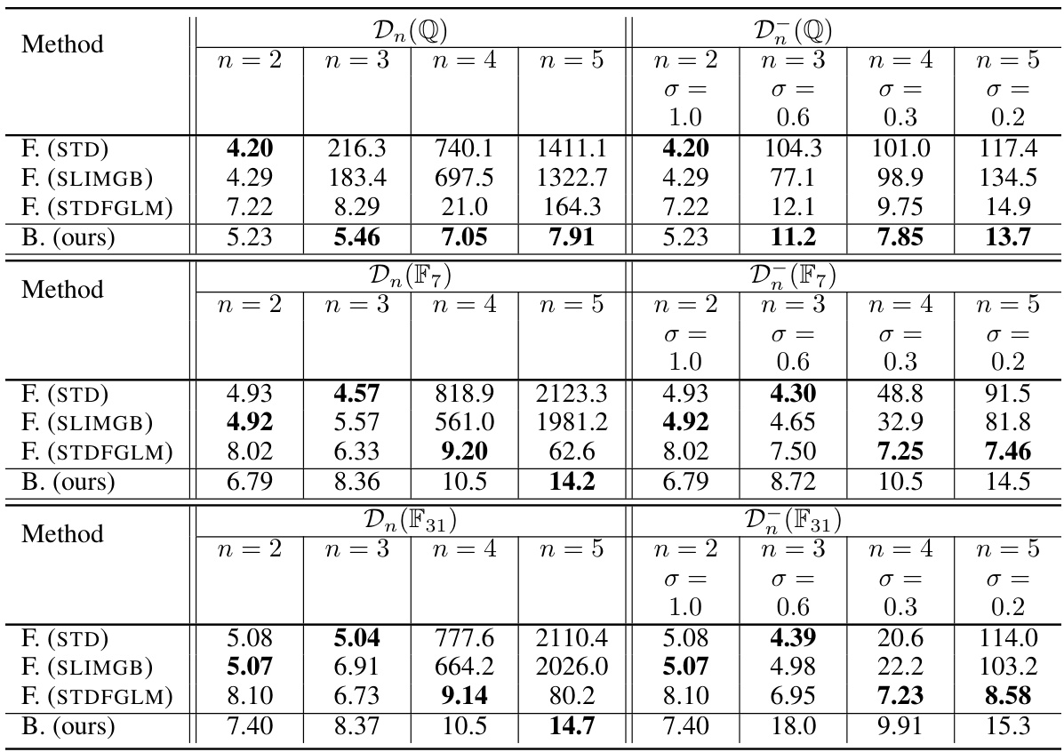
This table compares the runtime of forward and backward generation methods for creating datasets of Gröbner basis computation. The forward generation uses three different algorithms from SageMath, while the backward generation uses the authors’ proposed method. The table shows the runtime for datasets with varying numbers of variables (n=2, 3, 4, 5). The results indicate that the authors’ backward generation method is significantly faster than the forward generation methods, especially as the number of variables increases.

This table presents the success rate of forward generation using three different algorithms (STD, SLIMGB, STDFGLM) for generating Gröbner bases, with a timeout limit of 5 seconds. The success rate is calculated for different values of (n) (number of variables) and (\sigma) (density) for different coefficient fields ((\mathbb{Q}), (\mathbb{F}7), (\mathbb{F}{31})). A success is defined as a Gröbner basis computation that completes within the 5-second time limit. The table shows how the success rate varies based on the number of variables, the density of the polynomials, and the coefficient field.
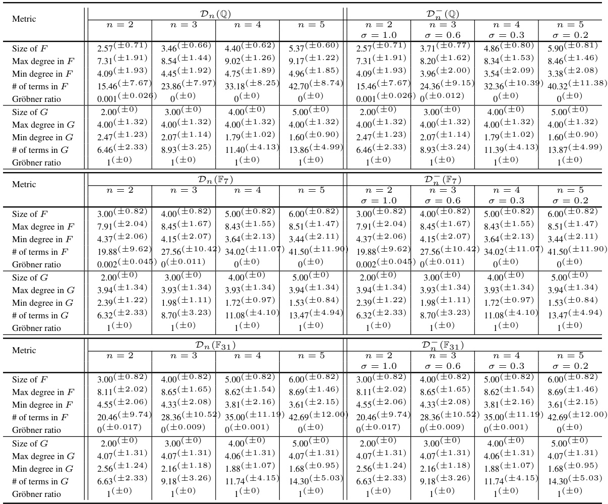
This table presents the accuracy and support accuracy of Gröbner basis computation using Transformers. The accuracy is measured based on whether the computed Gröbner basis is exactly correct. The support accuracy measures if only the terms of the polynomials are correct. Two different input embeddings are compared, discrete and hybrid, while performance is evaluated on different fields (Q, F7, F31) and varying numbers of variables (n). The density of the polynomials in the datasets is controlled via the parameter σ.
This table presents the accuracy and support accuracy of Gröbner basis computation by Transformers. It shows results using two different input embedding methods (discrete and hybrid) and across various coefficient fields (Q, F7, F31, R). The support accuracy measures the correctness of the terms (monomials) in the predicted Gröbner bases, even if the coefficients are slightly off. Datasets for different numbers of variables (n=2,3,4,5) are used, with the density (σ) of the polynomials varied for n=3,4,5.

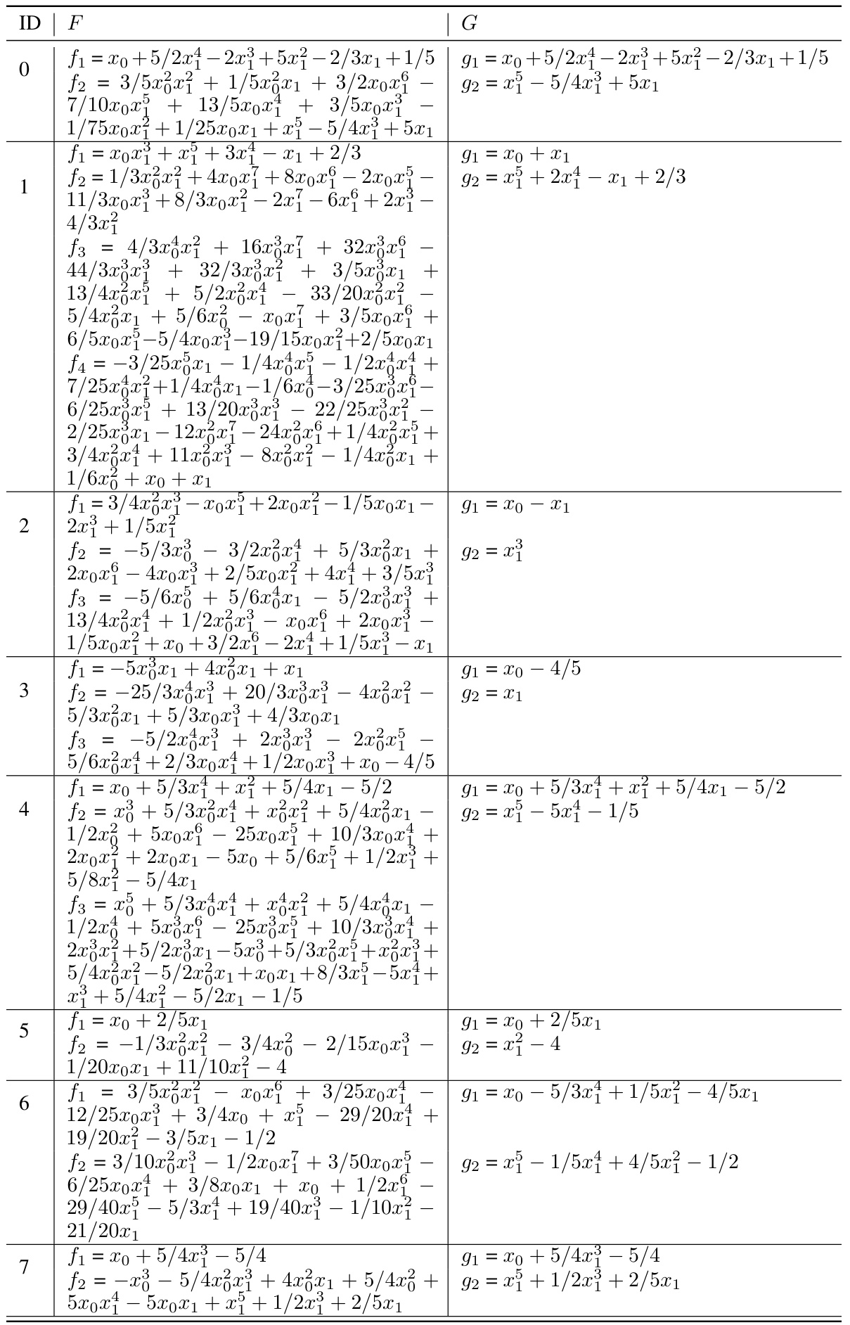
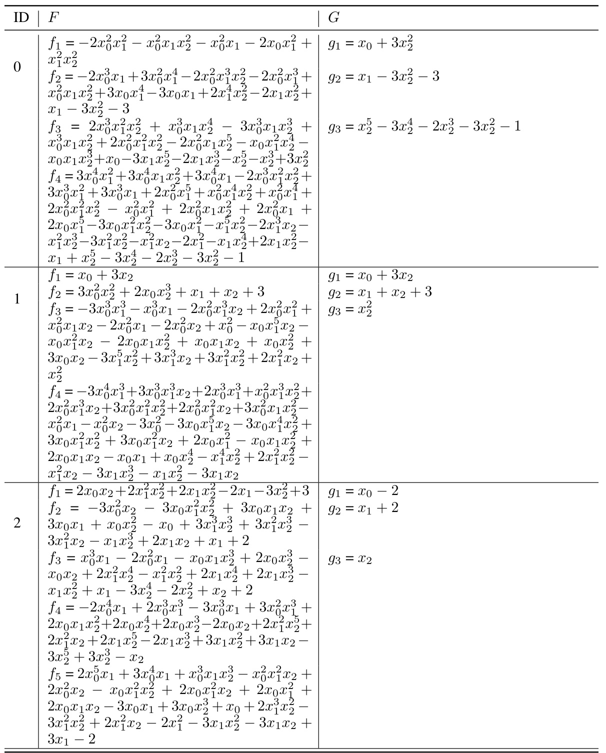
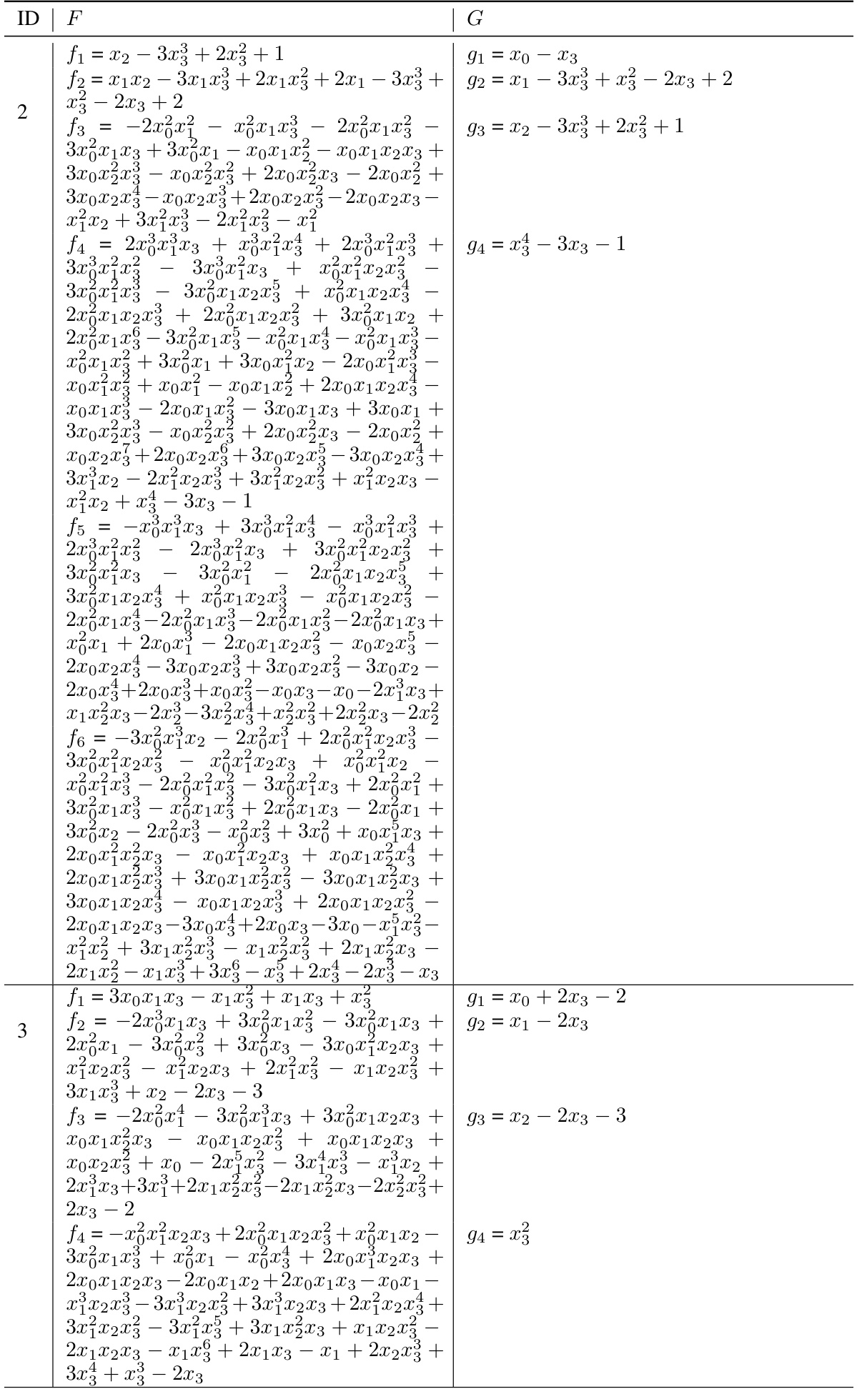
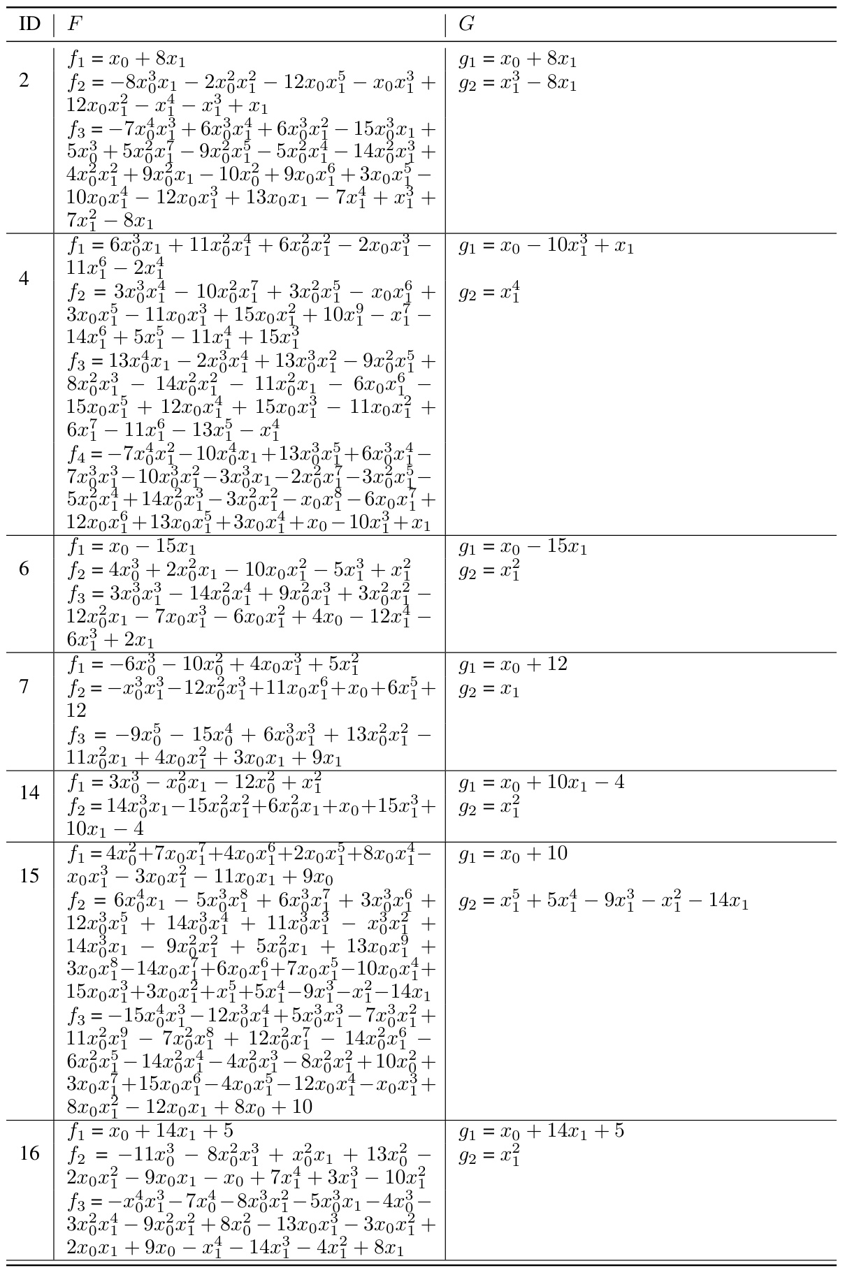
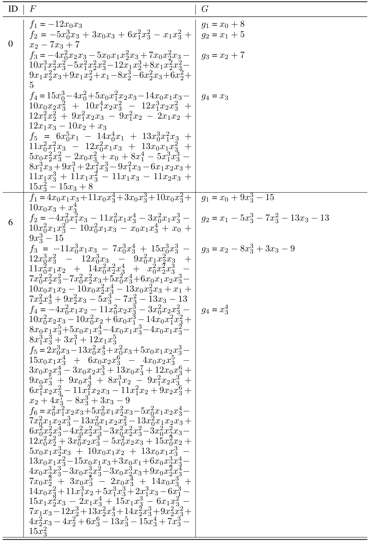
This table shows successful examples from the D₂(Q) test set, which contains pairs of non-Gröbner sets and Gröbner bases. For each example, the ID, the non-Gröbner set F, and its corresponding Gröbner basis G are listed. The table demonstrates that the Transformer model is able to correctly identify the Gröbner basis for these specific polynomial systems.

This table presents the accuracy and support accuracy of Gröbner basis computation using Transformers. The accuracy is measured for different coefficient fields (Q, F7, F31) and polynomial system sizes (n=2, 3, 4, 5). Two different input embedding methods are compared: discrete and hybrid. The hybrid embedding incorporates continuous values for the coefficients. Support accuracy focuses only on the correct identification of the terms in the Gröbner basis. The datasets used for n=3, 4, 5 are generated using a specific method (Alg. 1) with varying densities (σ).
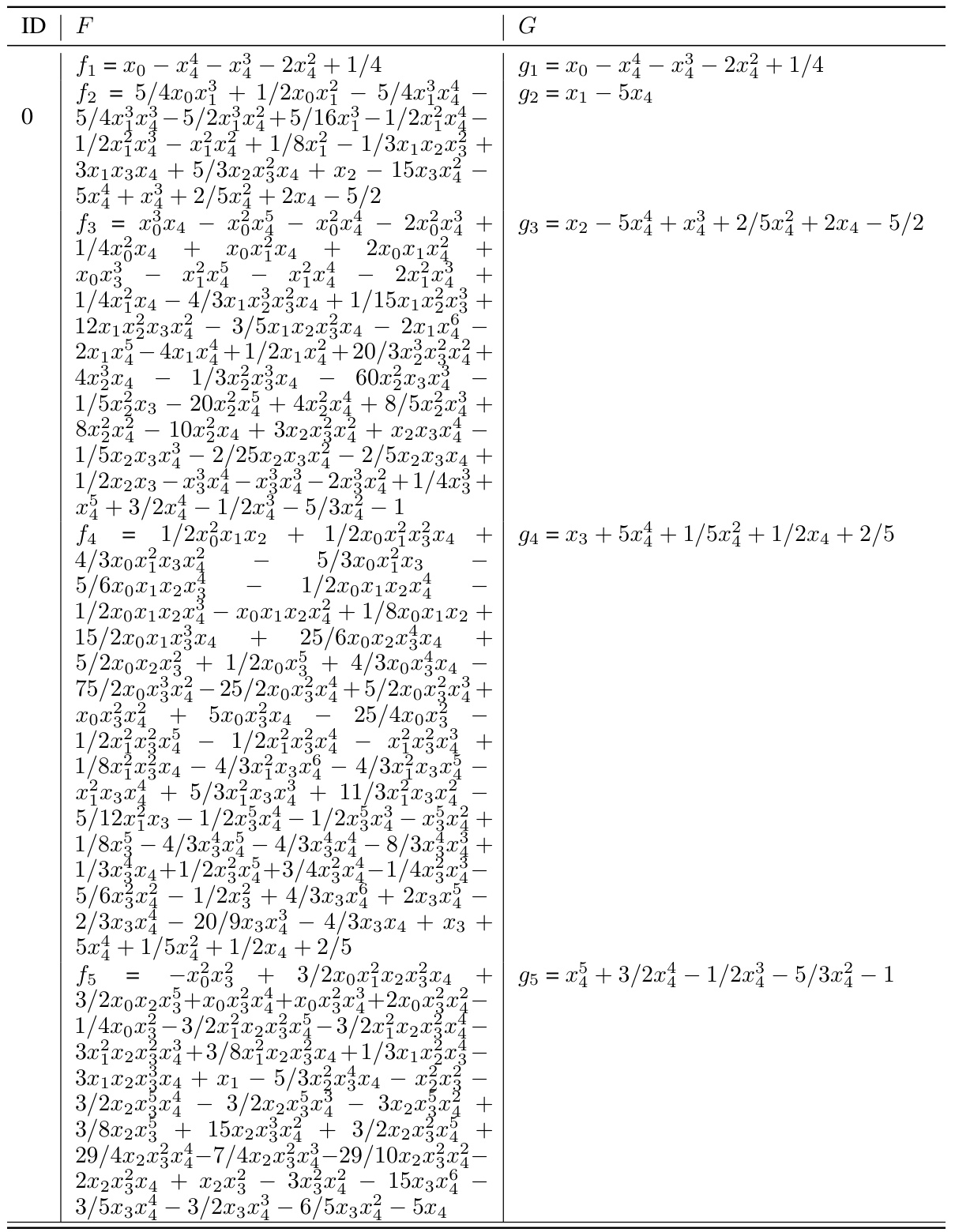
This table presents the accuracy and support accuracy of Gröbner basis computation using Transformers. The accuracy reflects how often the model correctly computed the entire Gröbner basis. The support accuracy measures how often the model correctly identified the terms (variables and exponents) present in the Gröbner basis, even if the coefficients were slightly off. Two different input embedding methods (discrete and hybrid) are compared, and results are shown for different coefficient fields (Q, F7, F31, R) and numbers of variables (n=2, 3, 4, 5). The datasets used for n=3, 4, and 5 were generated with varying densities (σ) to control complexity.
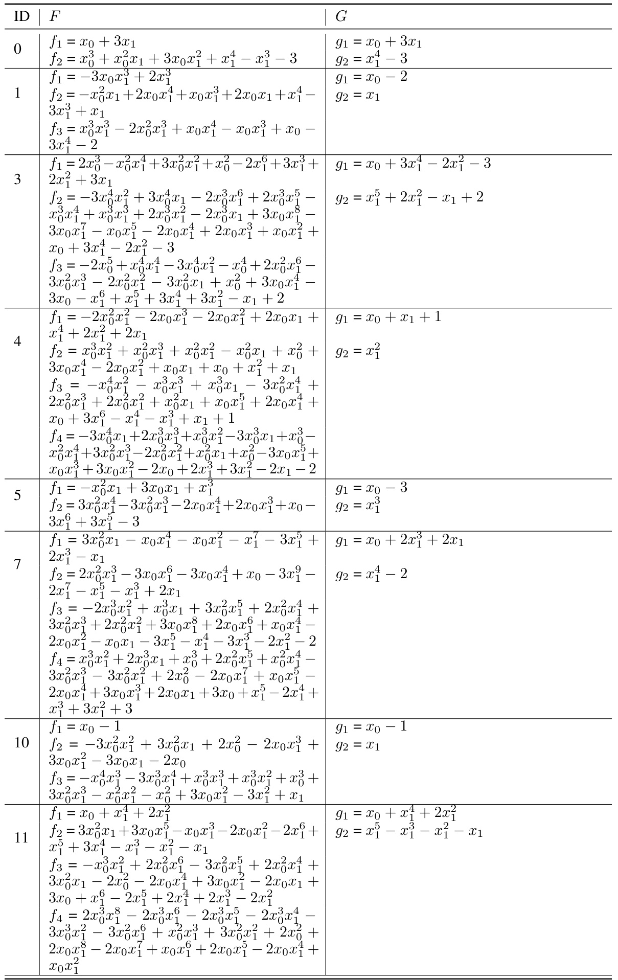
This table presents the accuracy and support accuracy of the Transformer model in computing Gröbner bases for different datasets (D(k)). The accuracy reflects how often the model correctly predicts the entire Gröbner basis. The support accuracy measures how often the model correctly predicts the terms (support) of the polynomials in the Gröbner basis, even if the coefficients are incorrect. The model was trained using both discrete and hybrid input embeddings. Different dataset sizes (n = 2, 3, 4, 5) are used and the density (σ) of the datasets varies across different values.
This table presents the accuracy and support accuracy of Gröbner basis computation using Transformers. The results are broken down by coefficient field (Q, F7, F31), the number of variables (n=2,3,4,5), and the type of input embedding used (discrete or hybrid). Support accuracy refers to correctly identifying the terms in the polynomials, regardless of whether the coefficients are perfectly predicted. The table notes that for n=3,4, and 5, the datasets are generated with specific densities (σ) using Algorithm 1.
This table presents the accuracy and support accuracy of Gröbner basis computation using Transformers. The results are shown for different coefficient fields (Q, F7, F31) and different polynomial system sizes (n=2, 3, 4, 5). Two different input embedding methods are compared: discrete input embedding and a hybrid embedding. The hybrid embedding combines discrete and continuous representations of numbers. The table shows that the model achieves high accuracy on the datasets but has difficulty with finite fields.

This table presents the accuracy and support accuracy of Gröbner basis computation by Transformers. The accuracy reflects how often the Transformer correctly computes the entire Gröbner basis, while the support accuracy measures how often it correctly identifies the terms (support) of the polynomials in the Gröbner basis. Two different input embedding methods are compared: discrete and hybrid. The results are broken down by coefficient field (Q, F7, F31) and number of variables (n=2,3,4,5). Note that the dataset generation method (Alg. 1) uses different densities (σ) for datasets with n=3, 4, and 5.
This table presents the accuracy and support accuracy of Gröbner basis computation using Transformers. The results are broken down by coefficient field (Q, F7, F31, R) and whether a discrete or hybrid input embedding was used during training. Support accuracy specifically measures the correctness of the polynomial’s terms, regardless of coefficient accuracy.

This table presents the accuracy and support accuracy of the Gröbner basis computation using Transformers. The accuracy is the percentage of correctly computed Gröbner bases, while the support accuracy measures the correctness of the terms (support) of the predicted Gröbner bases. Two different input embeddings are compared: discrete and hybrid. The results are shown for different coefficient fields (Q, F7, F31) and polynomial dimensions (n = 2, 3, 4, 5). Datasets for n>2 are generated using a specific method (U1,U2 from Algorithm 1) with varying densities.
This table presents the accuracy and support accuracy of Gröbner basis computation by Transformers. The models were trained using either discrete or hybrid input embedding methods. The accuracy is the percentage of correctly predicted Gröbner bases, and the support accuracy considers two polynomials identical if they have the same terms, regardless of coefficients. The datasets used (D(k)) varied in the number of variables (n) and coefficient fields (k), and different densities (σ) were employed for the larger datasets.

This table presents the accuracy and support accuracy of Gröbner basis computation using Transformers. The results are broken down by coefficient field (Q, F7, F31), the dimensionality of the polynomial system (n=2,3,4,5), and the type of input embedding used (discrete or hybrid). Support accuracy measures the accuracy of predicting the terms (support) of the polynomials in the Gröbner basis, even if the coefficients are incorrect. The table also notes that datasets for n>2 used a specific generation method (Alg 1, with varying densities).
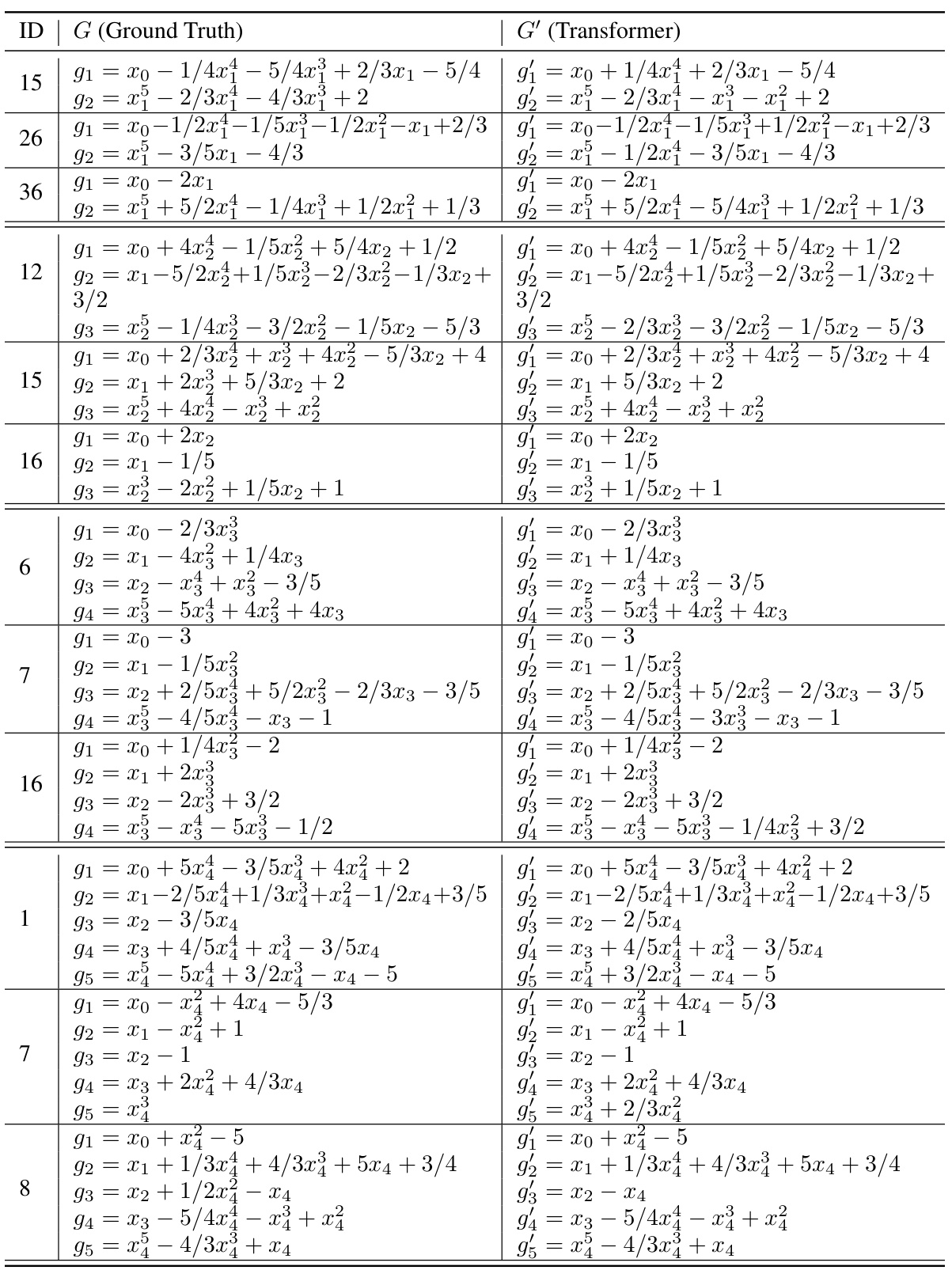
This table shows the accuracy and support accuracy of the Transformer model in computing Gröbner bases for different datasets (D(k)). The accuracy represents the overall correctness of the generated Gröbner basis, while support accuracy measures the correctness of the terms (variables and exponents) in the generated Gröbner basis, even if the coefficients are slightly off. Two training methods are compared: discrete input embedding and hybrid input embedding. The datasets used for n=3, 4, and 5 are generated using a specific method (Alg. 1) with varying density parameters (σ).
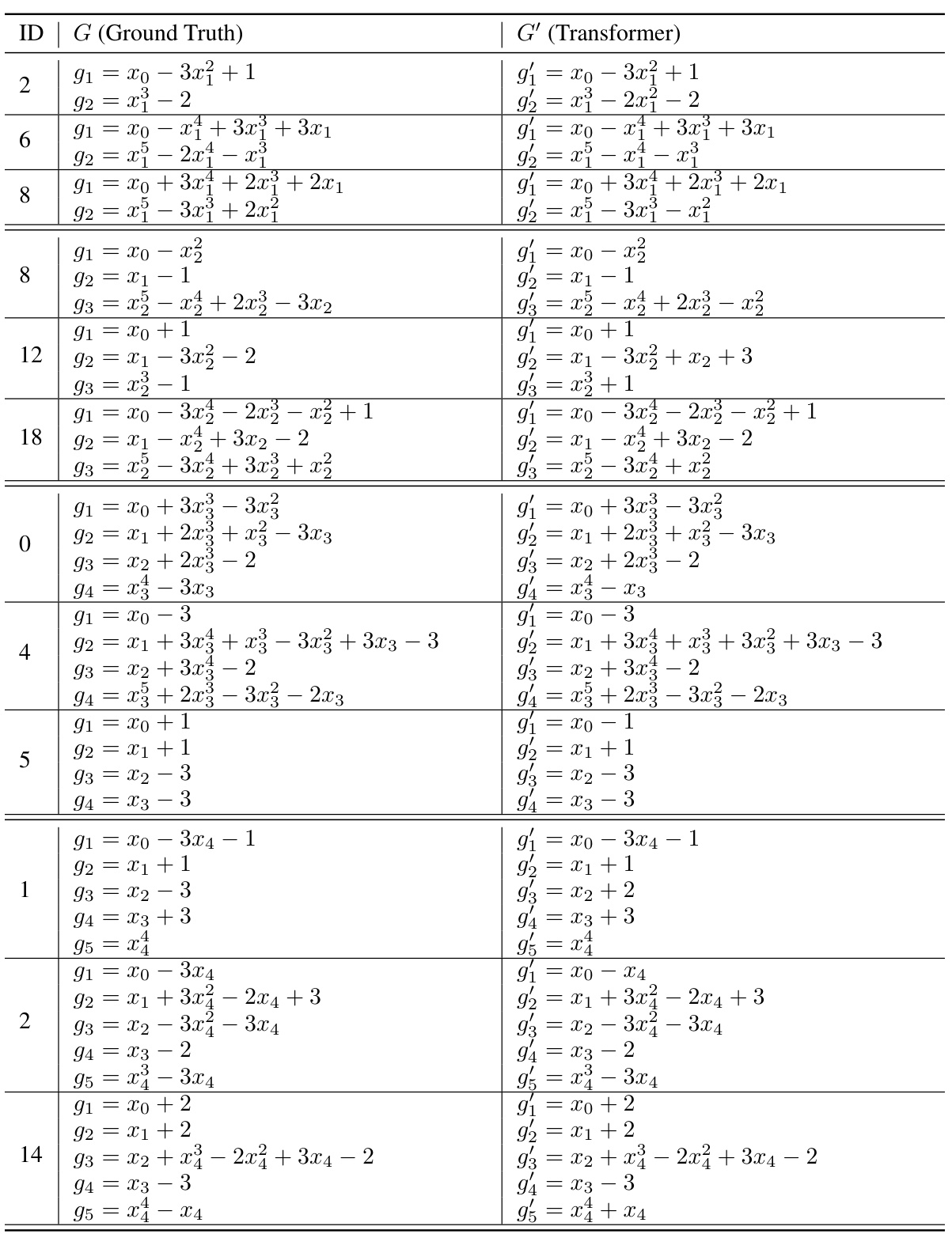
This table presents the accuracy and support accuracy of Gröbner basis computation using Transformers. The results are broken down by coefficient field (Q, F7, F31, R) and input embedding method (discrete or hybrid). Support accuracy measures the correctness of the polynomial terms, while accuracy accounts for both terms and coefficients. The table shows that performance varies across different coefficient fields and embedding techniques, with generally higher accuracy on infinite fields (Q, R) compared to finite fields (F7, F31).

This table presents the accuracy and support accuracy of Gröbner basis computation using Transformers. The model is trained using either discrete or hybrid input embeddings. Support accuracy is based on the polynomials’ terms only, regardless of coefficients. The dataset density is varied for n=3,4,5.

This table compares the runtime of forward and backward generation methods for Gröbner basis computation. The forward generation uses three different algorithms from SageMath, while the backward generation uses the proposed method. The table shows that the backward method is significantly faster than the forward methods, especially as the number of variables (n) increases. Timeout instances are also noted.

This table presents the accuracy and support accuracy of Gröbner basis computation using Transformers. The results are shown for different coefficient fields (Q, F7, F31) and polynomial dimensions (n=2, 3, 4, 5). Two training methods are compared: discrete input embedding and hybrid embedding. Support accuracy measures how well the Transformer predicts the terms in the Gröbner basis, even if the coefficients are incorrect.

This table presents the accuracy and support accuracy of Gröbner basis computation using Transformers. The results are categorized by the coefficient field (Q, F7, F31), the input embedding method (discrete or hybrid), and the number of variables (n=2,3,4,5). Support accuracy refers to the percentage of correctly predicted polynomial supports (sets of terms), irrespective of the coefficient values. The density (σ) values indicate the sparsity level of the polynomials in the datasets.
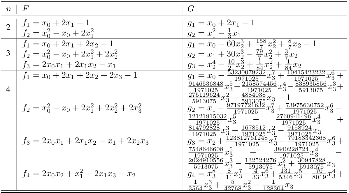
This table presents the accuracy and support accuracy of Gröbner basis computation using Transformers. The results are broken down by coefficient field (Q, F7, F31, R) and input embedding method (discrete and hybrid). Support accuracy measures the accuracy of predicting the terms (support) in the Gröbner basis, even if the coefficients are not perfectly predicted. The datasets used for n=3, 4, and 5 were generated using a specific method (Alg. 1) with varying densities (σ).
Full paper#
