↗ OpenReview ↗ NeurIPS Homepage ↗ Chat
TL;DR#
Deep learning models often struggle with dataset bias, where spurious correlations in training data lead to poor generalization. Existing methods attempt to identify and leverage bias-conflicting samples, but struggle with accurate detection due to the inherent difficulty in distinguishing them from other samples. This challenge is particularly pressing because mislabeled samples and bias-conflicting samples exhibit striking similarities.
This paper tackles this challenge by drawing parallels between mislabeled sample detection and bias-conflicting sample detection. It leverages influence functions, a standard method for mislabeled sample detection, to identify and utilize bias-conflicting samples. The study introduces a new technique called Bias-Conditioned Self-Influence (BCSI) to improve detection, and proposes a fine-tuning remedy using a small pivotal set constructed from BCSI to effectively rectify biased models. Experiments show BCSI significantly boosts detection precision and the fine-tuning strategy effectively corrects bias in various datasets, even after other debiasing techniques have been applied. The proposed method is both simple and highly effective.
Key Takeaways#
Why does it matter?#
This paper is important because it offers a novel, effective, and complementary approach to address dataset bias, a critical problem in machine learning. It improves the precision of bias detection, rectifies biased models effectively, and works well even with models already debiased by existing techniques. This opens new avenues for research on fairness and robustness in AI.
Visual Insights#

This figure compares the precision of four different methods in detecting bias-conflicting samples across four different datasets: CMNIST, CIFAR10C, BFFHQ, and Waterbird. The methods compared are using the loss value, gradient norm, influence function on the training set, and self-influence. The precision is calculated against a ground truth of bias-conflicting samples. The bar chart shows the average precision across three runs for each method and dataset.

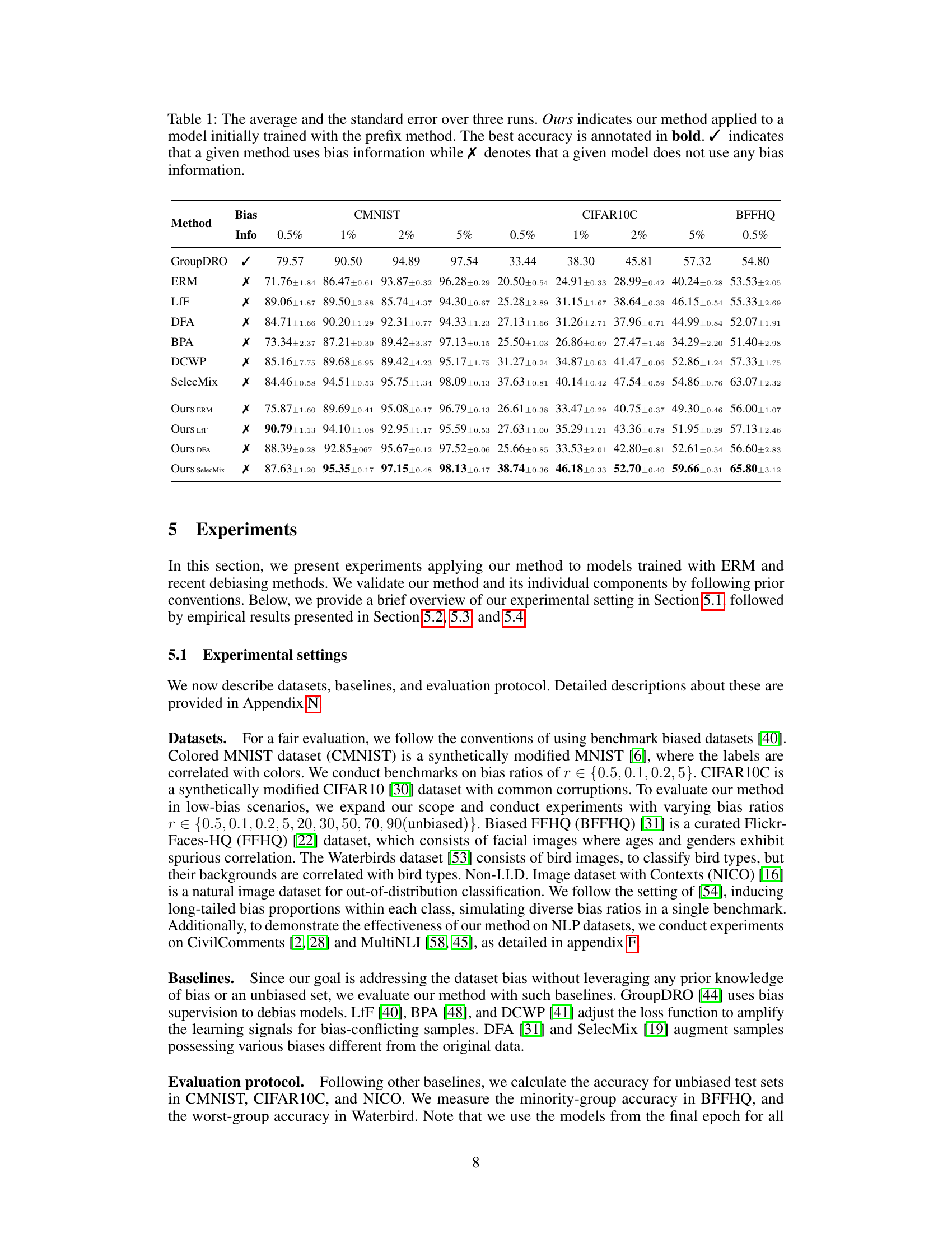
This table presents the average accuracy and standard error for various methods on three datasets (CMNIST, CIFAR10C, and BFFHQ) with different bias ratios. The ‘Bias Info’ column indicates whether the method utilizes bias information (✓) or not (X). The best accuracy for each setting is shown in bold. The ‘Ours’ rows show the results when the proposed method is applied on top of other methods.
In-depth insights#
Bias-Sample Detection#
The concept of ‘Bias-Sample Detection’ in this research paper is crucial for addressing dataset bias in machine learning. The core idea revolves around identifying samples that contradict the dominant spurious correlations learned by the model. This is achieved by leveraging influence functions, specifically Self-Influence (SI), a method typically used for mislabeled sample detection. The paper investigates the similarities and differences between mislabeled and bias-conflicting samples, highlighting the critical need for a nuanced approach that addresses the unique challenges of bias detection. The authors propose Bias-Conditioned Self-Influence (BCSI), which enhances the precision of bias-conflicting sample identification by carefully managing the model’s training process to emphasize learning of spurious correlations. This refined detection method is then used to construct a pivotal subset of samples for fine-tuning the model, effectively rectifying the bias. The focus on leveraging existing techniques (influence functions) in a novel way is a significant contribution, demonstrating the potential for simple yet effective solutions to complex problems in machine learning. The paper emphasizes that this approach is complementary to existing debiasing techniques, leading to further performance improvements.
Self-Influence Analysis#
A self-influence analysis within a research paper investigating dataset bias would likely involve a detailed examination of how individual data points affect a model’s predictions, particularly focusing on identifying bias-conflicting samples. This analysis would use a technique like Influence Functions, measuring the impact of removing a single sample on the model’s prediction of that same sample. High self-influence would indicate a sample’s significant effect, suggesting it is a bias-conflicting sample contradicting the model’s learned bias. The analysis would likely compare self-influence scores across different samples to pinpoint those that deviate significantly from the norm. This would likely involve visualizations such as histograms to illustrate the distribution of self-influence scores, helping identify and differentiate between bias-aligned and bias-conflicting samples. The core contribution would be the method’s efficacy in precisely identifying these bias-conflicting samples, which is crucial for subsequent debiasing interventions. The analysis would also likely include exploring the conditions under which self-influence is most effective for identifying bias-conflicting samples.
BCSI Fine-tuning#
The proposed BCSI fine-tuning method offers a novel approach to debiasing models by leveraging the identified bias-conflicting samples. Instead of relying on external unbiased data or complex procedures, it uses a small, carefully selected subset (pivotal set) enriched with bias-conflicting samples, created using the BCSI metric. This pivotal set guides the fine-tuning process, effectively counteracting the learned spurious correlations. The method’s simplicity and efficacy are highlighted by its complementary nature; it enhances performance even when applied to models already processed by other debiasing techniques. The reliance on self-influence avoids the need for an external validation set, significantly simplifying the debiasing process. Fine-tuning with this pivotal set shows improved performance across a range of bias severities, indicating the approach’s robustness. However, limitations exist regarding its dependence on the accurate identification of bias-conflicting samples by BCSI and sensitivity to the size of the pivotal set. Further research is needed to optimize pivotal set selection and explore its broader applicability across diverse datasets and model architectures.
Method Limitations#
The method’s reliance on identifying bias-conflicting samples using Bias-Conditioned Self-Influence (BCSI) introduces limitations. BCSI’s effectiveness depends on the model’s early training phase, where bias is prioritized over task-relevant features. This is not always the case, so the accuracy of the pivotal set creation may vary. Furthermore, the approach’s reliance on a small pivotal subset for fine-tuning may overfit to specific characteristics of this subset and may not generalize well to unseen data. The method’s performance also depends on the dataset’s bias severity; it performs better with highly biased datasets but may struggle with low-bias ones. Lastly, it is worth noting that the computational cost, although reduced compared to full model retraining, could still be an issue for very large datasets.
Future Directions#
Future research could explore extending the self-influence approach to other types of bias beyond those studied. Investigating how to automatically identify the optimal epoch for BCSI calculation without manual tuning would improve usability and efficiency. Combining BCSI with other debiasing methods may lead to synergistic improvements. Further research might delve into the theoretical underpinnings of BCSI, potentially developing tighter bounds on its effectiveness or exploring alternative ways to quantify bias-conflicting samples. The scalability and generalizability of the approach to very large datasets and more complex models require investigation. Addressing fairness concerns head-on by explicitly designing metrics to assess the fairness of the model after using BCSI is crucial for ensuring responsible AI. Finally, it would be insightful to conduct an extensive comparison with other state-of-the-art bias mitigation methods across diverse datasets and bias types.
More visual insights#
More on figures
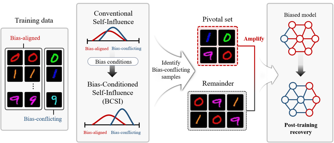
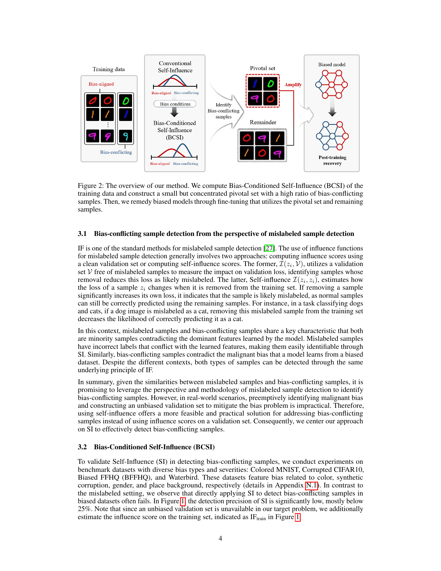
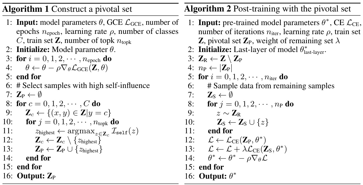
This figure illustrates the proposed method’s workflow. First, Bias-Conditioned Self-Influence (BCSI) is calculated for the training data to identify bias-conflicting samples. A pivotal set is created using these samples, which is then used in a fine-tuning process along with the remaining samples to remedy the biased model. The method aims to improve the precision of detecting bias-conflicting samples and effectively rectify biased models.

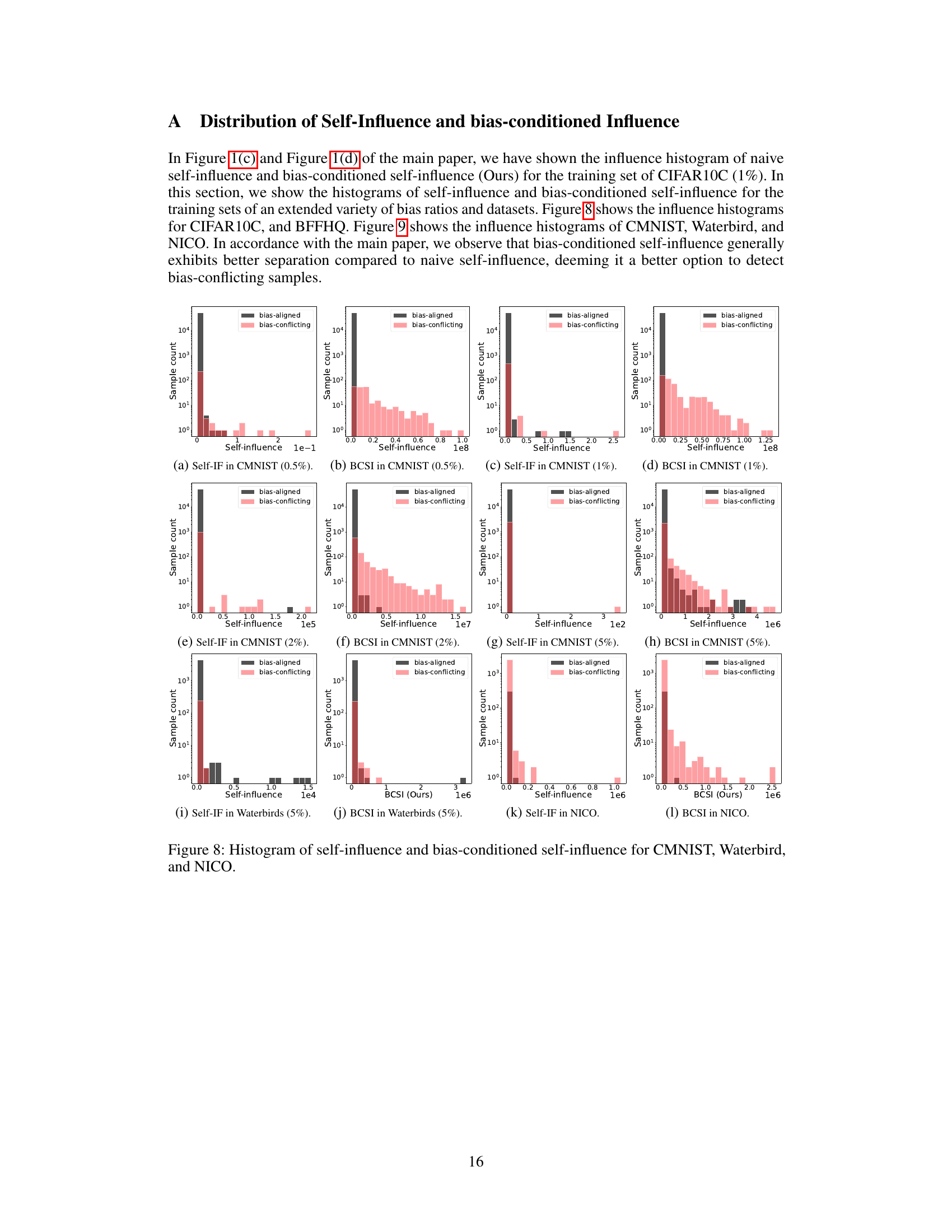
This figure presents a comprehensive analysis of influence functions on biased datasets. It shows how classification accuracy changes over training epochs for both bias-aligned and bias-conflicting samples. It also compares the detection precision of two influence function methods (IFtrain and SI) under varying ratios of bias-conflicting samples in the CIFAR10C dataset. Finally, it visualizes the distribution of self-influence scores for both bias-aligned and bias-conflicting samples using histograms.

This figure compares the precision of four different methods in detecting bias-conflicting samples: Loss, Gradient Norm, Influence Function on the training set (IFtrain), and Self-Influence (SI). The precision is calculated against the ground truth number of bias-conflicting samples. The bar chart displays the average precision across three separate runs for each method, showcasing their relative effectiveness in identifying such samples. The datasets used are CMNIST (1%), CIFAR10C (1%), BFFHQ, and Waterbird.
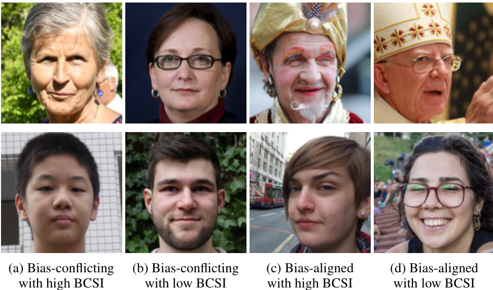
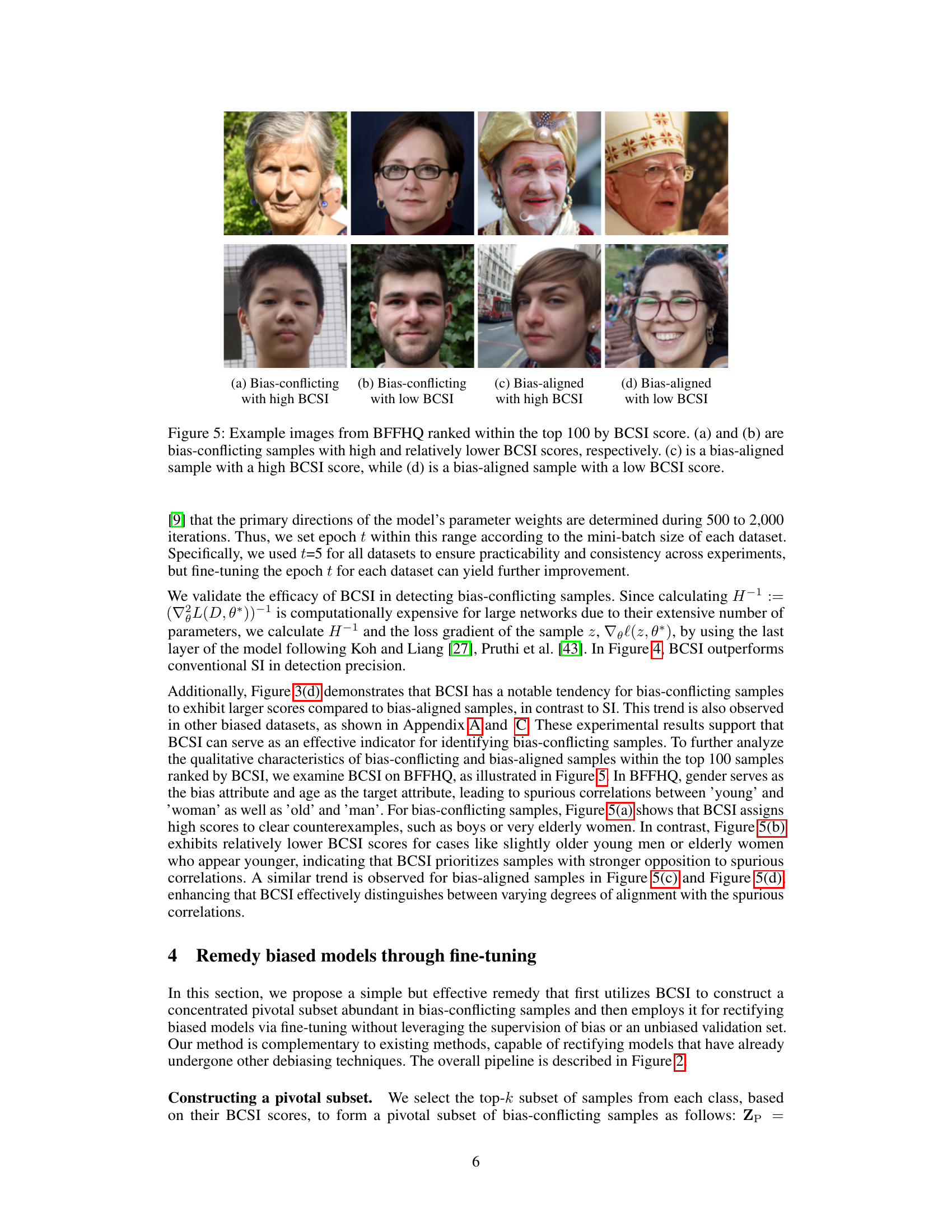
This figure shows example images from the Biased FFHQ dataset, which are ranked by their Bias-Conditioned Self-Influence (BCSI) scores. The top row displays examples of images with high BCSI scores and the bottom row examples with low BCSI scores. Within each row, the left side shows bias-conflicting samples and the right side bias-aligned samples. The image examples visually illustrate how BCSI can better distinguish bias-conflicting samples (those contradicting the learned bias) from bias-aligned samples, which helps in identifying and rectifying model bias.

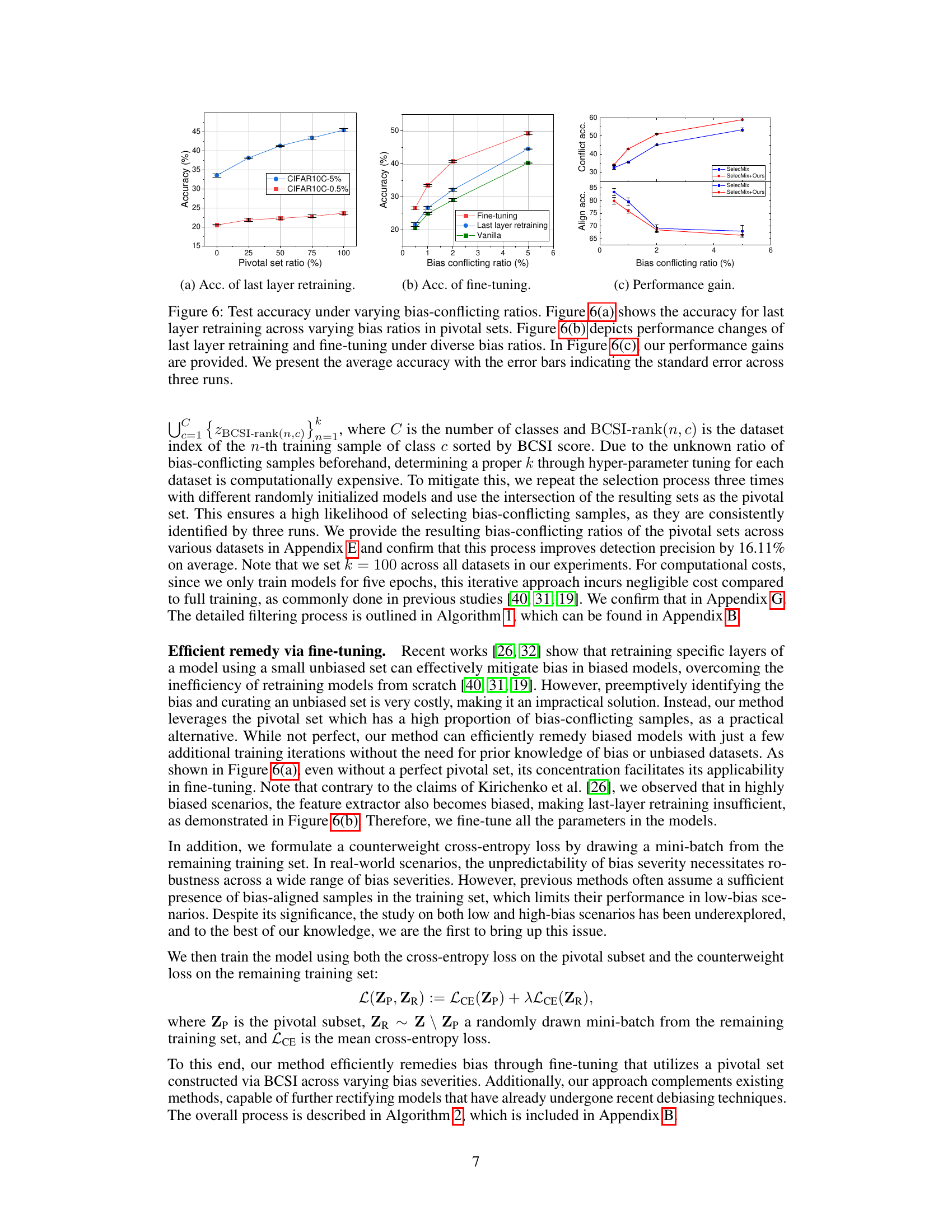
This figure shows the results of experiments conducted to evaluate the performance of the proposed method for rectifying biased models. Three subfigures present different aspects of the model’s performance across various conditions. (a) shows the accuracy of retraining only the last layer of the model using pivotal sets with different ratios of bias-conflicting samples. (b) compares the accuracy of retraining the last layer, fine-tuning the entire model, and using a vanilla model without any bias correction methods. This comparison is done across varying bias-conflicting ratios. (c) illustrates the performance gain achieved by incorporating the proposed method into SelecMix. The x-axis represents the bias conflicting ratio in all subfigures. Error bars show standard errors across three runs.

This figure compares the performance of four different methods (Loss, Gradient Norm, Influence Function on training set, and Self-Influence) for detecting bias-conflicting samples in four different datasets (CMNIST, CIFAR10C, BFFHQ, and Waterbird). The precision of each method is shown as a bar chart, with error bars indicating the standard deviation across three runs. The results show that Self-Influence performs better than the other methods for detecting bias-conflicting samples in most cases.
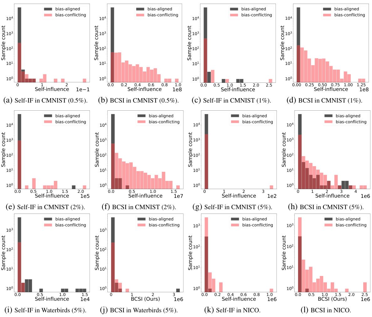
This figure compares the precision of four different methods in detecting bias-conflicting samples across four different datasets: CMNIST, CIFAR10C, BFFHQ, and Waterbird. The four methods are: Loss (using the loss value), Gradient Norm (using gradient norm), Influence Function on training set (IF_train), and Self-Influence (SI). The bar chart shows the average precision across three runs for each method and dataset. The results show that Self-Influence (SI) generally performs better than the other methods in identifying bias-conflicting samples, highlighting its potential use in addressing dataset bias.
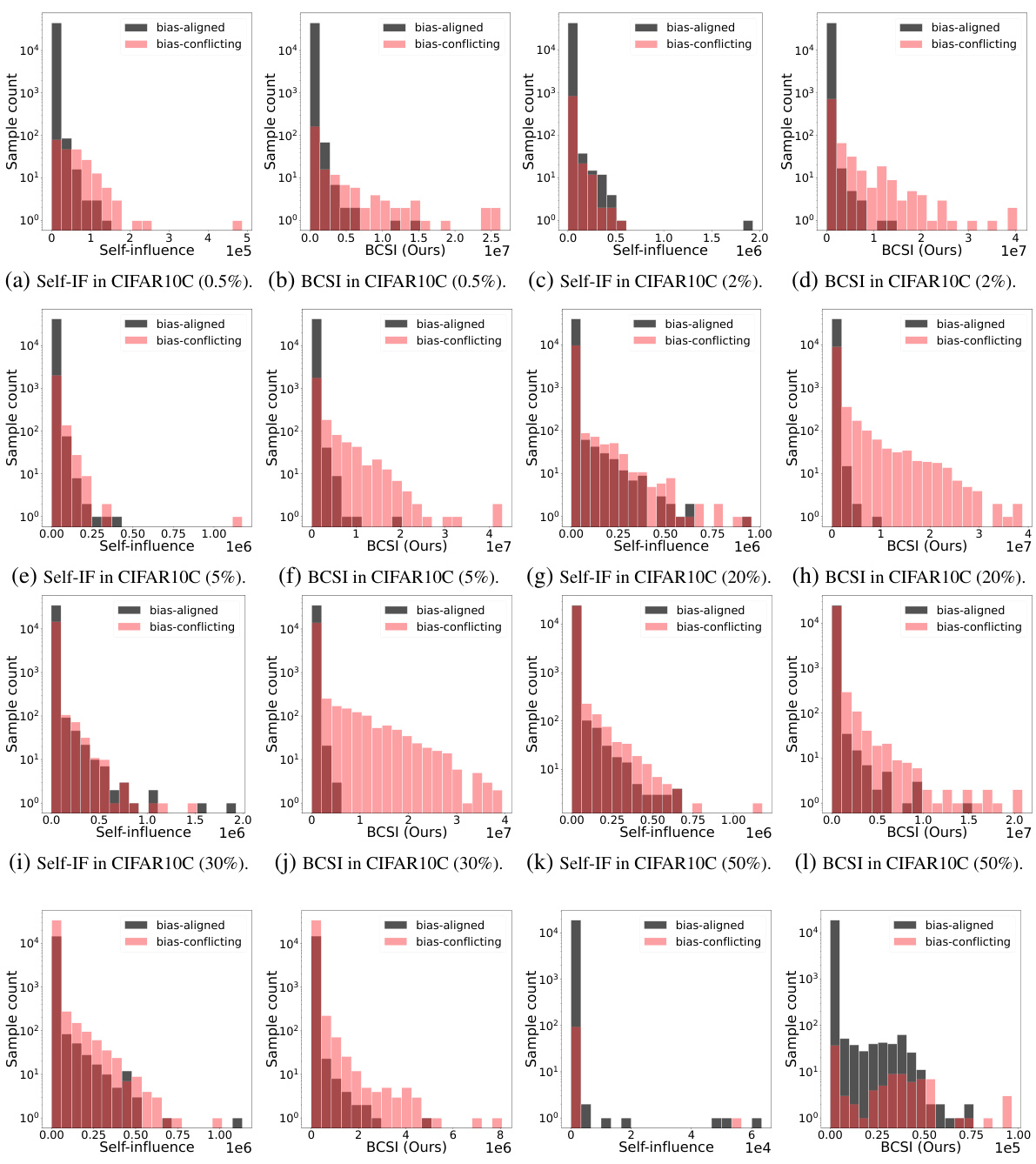
This figure compares the performance of four different methods (Loss, Gradient Norm, Influence Function on training set, and Self-Influence) for detecting bias-conflicting samples in four different datasets (CMNIST, CIFAR10C, BFFHQ, and Waterbird). The precision of each method is calculated using the ground truth number of bias-conflicting samples. The bars represent the average precision across three runs for each method and dataset. The results show that Self-Influence generally performs better than the other methods for detecting bias-conflicting samples.

This figure displays the test accuracy under varying bias-conflicting ratios. The leftmost subplot (a) shows the accuracy for last layer retraining across various bias ratios in pivotal sets. The middle subplot (b) compares the performance changes of last layer retraining and fine-tuning. The rightmost subplot (c) presents performance gains. Error bars represent the standard error across three runs. It demonstrates the effectiveness of the proposed method for rectifying biased models under various bias-conflicting ratios, especially highlighting the complementary nature of fine-tuning to existing methods.

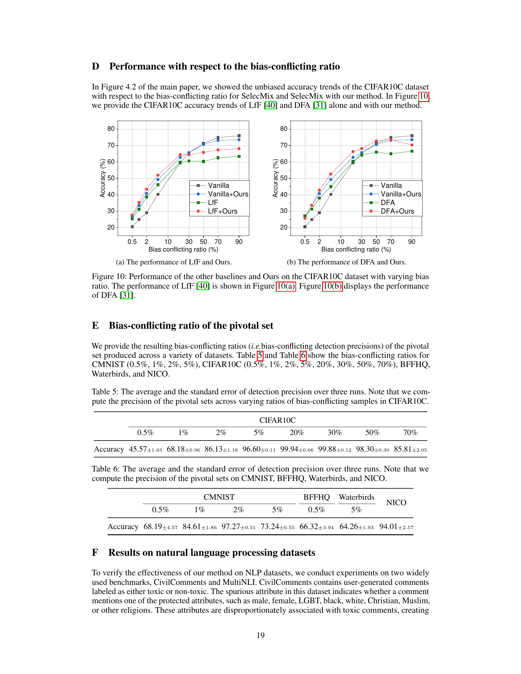
This figure shows the performance comparison of applying the proposed method to other debiasing methods such as LfF and DFA with varying bias-conflicting ratios. The x-axis shows the bias-conflicting ratio, while the y-axis represents the accuracy. The results demonstrate the effectiveness of the proposed method across different bias levels when combined with existing approaches.
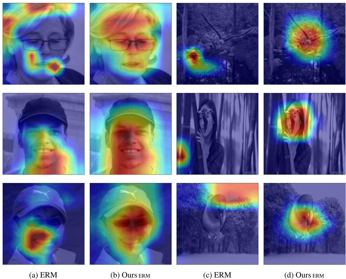
This figure compares the precision of four different methods (Loss, Gradient Norm, Influence Function on training set, and Self-Influence) in detecting bias-conflicting samples across four different datasets (CMNIST, CIFAR10C, BFFHQ, and Waterbird). The precision is calculated using the ground truth number of bias-conflicting samples. The bar chart displays the average precision across three runs for each method and dataset. The results show that Self-Influence generally outperforms the other methods.

This figure compares the precision of four different methods in detecting bias-conflicting samples across four datasets: CMNIST, CIFAR10C, FFHQ, and Waterbird. The methods are: using the training loss, the gradient norm, the influence function evaluated on the training set (IF_train), and self-influence (SI). The precision is calculated using the ground truth number of bias-conflicting samples. The bar graph shows the average precision across three runs for each method on each dataset. It highlights that Self-Influence (SI) generally performs poorly compared to other methods.

This figure compares the precision of four different methods in detecting bias-conflicting samples across four different datasets. The methods are loss-based, gradient norm-based, influence function-based on the training set, and self-influence-based. The results are presented as bar graphs showing the average precision for each method across three runs, highlighting the relative effectiveness of Self-Influence in identifying bias-conflicting samples compared to other methods.
More on tables
This table presents the average accuracy and standard error over three runs for various debiasing methods on four different datasets (CMNIST, CIFAR10C, BFFHQ, Waterbird) with different bias ratios. The ‘Ours’ methods represent the authors’ proposed method applied after each of the other methods (ERM, LfF, DFA, SelecMix). The table also indicates whether each method uses bias information or not.
This table presents the average accuracy and standard error achieved by various methods on different datasets (CMNIST, CIFAR10C, BFFHQ) with varying levels of bias (0.5%, 1%, 2%, 5%). The methods compared include ERM (Empirical Risk Minimization), several debiasing methods (GroupDRO, LfF, DFA, SelecMix), and the proposed method (‘Ours’) applied to models pre-trained with different methods. The table shows how the proposed method improves the accuracy of other debiasing methods, especially at higher bias levels, and its competitiveness to ERM, a baseline approach that does not explicitly attempt to remove bias.

This table presents the performance comparison of two methods in detecting bias-conflicting samples across various datasets. Self-Influence (SI) and Bias-Conditioned Self-Influence (BCSI) are compared. The precision, which is the ratio of correctly identified bias-conflicting samples to the total number of bias-conflicting samples, is calculated for each dataset and bias ratio. The average precision and its standard error across three runs are reported for a more robust assessment of each method’s performance.

This table shows the average accuracy and standard error for different bias-handling methods on four benchmark datasets (CMNIST, CIFAR10C, BFFHQ, Waterbird). The results are shown for various bias ratios (0.5%, 1%, 2%, 5%). The ‘Ours’ methods represent the proposed method applied after other baseline methods. The presence or absence of bias information in each method’s training is also indicated. Bold values represent the highest achieved accuracy in each setting.

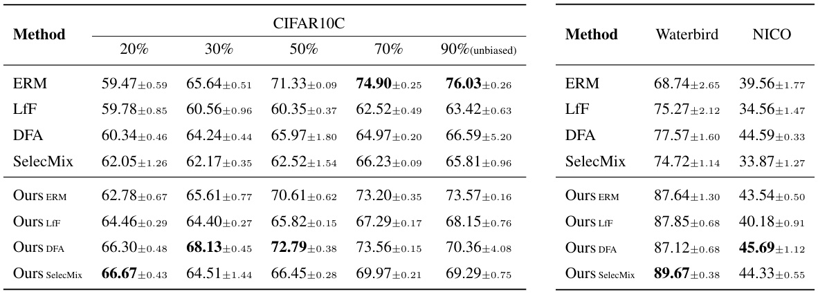
This table presents the average accuracy and standard error, across three runs, for various methods on low-bias scenarios using different datasets. The low-bias scenarios are defined by the bias-conflicting ratio in the datasets (ranging from 20% to 90% for CIFAR10C). The methods compared include ERM (Empirical Risk Minimization), LfF (Learning from Failure), DFA (Disentangled Feature Augmentation), SelecMix, and the proposed method combined with each of these baselines (Ours ERM, Ours LfF, Ours DFA, Ours SelecMix). The table aims to demonstrate the performance of the proposed method in low-bias settings, where existing debiasing methods may underperform.
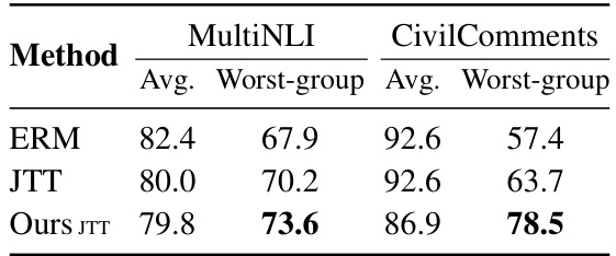
This table presents the average and worst-group accuracy results on two NLP datasets, MultiNLI and CivilComments, for different methods: ERM, JTT, and the proposed method combined with JTT. It demonstrates the effectiveness of the proposed method in improving the worst-group accuracy, particularly when used in conjunction with the JTT method. The ‘Avg.’ column represents the average accuracy across all groups, while ‘Worst-group’ represents the accuracy on the group with the lowest performance.

This table presents the average accuracy and standard error achieved by various methods on benchmark datasets with different bias levels. The methods are categorized as either using bias information or not. The ‘Ours’ method represents the proposed approach applied to models pre-trained with other methods. The best accuracy for each setting is highlighted in bold.

This table presents the average accuracy and standard error obtained by various methods (ERM, GroupDRO, LfF, DFA, BPA, DCWP, SelecMix, and Ours) on four benchmark datasets (CMNIST, CIFAR10C, BFFHQ, and Waterbirds) with different bias ratios. The ‘Ours’ column shows the results of the proposed method, both when applied to models trained with ERM and when applied to models already debiased by other methods. The best accuracy for each setting is highlighted in bold. A checkmark (✓) indicates that a method explicitly used bias information during training, while an ‘X’ denotes that it did not.

This table shows the average and standard error of the number of samples selected for the pivotal set across three different runs for varying numbers of intersections. The data is broken down by the percentage of bias-conflicting samples in the CIFAR10C dataset (0.5%, 1%, 2%, 5%, 20%, 30%, 50%, 70%). It demonstrates the effect of using multiple random model initializations on the size of the pivotal set.

This table compares the performance of different debiasing methods on four benchmark datasets (CMNIST, CIFAR10C, BFFHQ, Waterbird) with varying bias levels (0.5%, 1%, 2%, 5%). The methods include ERM (Empirical Risk Minimization), LfF (Learning from Failure), DFA (Disentangled Feature Augmentation), BPA (Bias-aware Pseudo-attribute), SelecMix, and the proposed method (‘Ours’). The table shows the average accuracy and standard error for each method across three runs. The ‘Ours’ results represent the proposed approach used alone and in conjunction with other methods. The ‘Info’ column indicates whether a method uses bias information (✓) or not (X). The bold values highlight the best accuracy for each setting.

This table compares the performance of different bias mitigation methods across four datasets (CMNIST, CIFAR10C, BFFHQ, Waterbirds) with varying bias ratios (0.5%, 1%, 2%, 5%). The methods include ERM (Empirical Risk Minimization), GroupDRO, LfF, DFA, BPA, DCWP, SelecMix, and the proposed method (Ours), applied both independently and in combination with other methods. The table shows the average accuracy and standard error for each method and dataset. The ‘Info’ column indicates whether each method utilizes bias information (✓) or not (X). Bold values represent the best-performing method for each combination.

This table presents the average accuracy and standard error over three runs for different bias mitigation methods on four benchmark datasets (CMNIST, CIFAR10C, BFFHQ, Waterbird). The results are categorized by bias ratio (0.5%, 1%, 2%, 5% for CMNIST and CIFAR10C; 0.5% for BFFHQ; 0.5%, 1%, 2%, 5% for Waterbird). The ‘Ours’ methods indicate the results when the proposed method is applied to models already pre-trained with other methods. The bold values represent the best performance for each setting. The ✓ and X symbols denote whether bias information was used by the method or not.
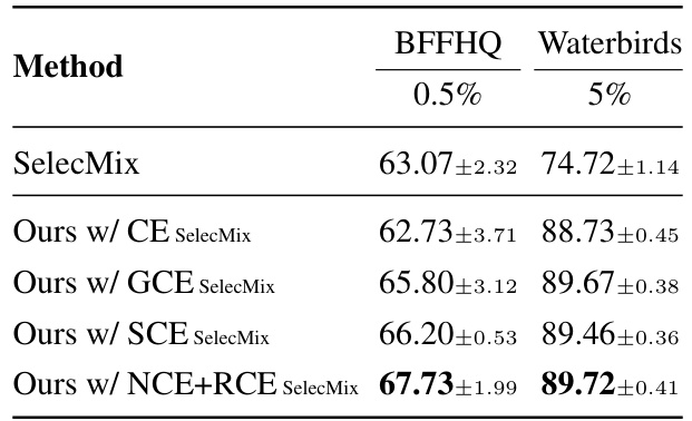
This table presents the average accuracy and standard error over three runs for different bias detection methods on four datasets: CMNIST, CIFAR10C, BFFHQ, and Waterbirds. The methods compared include ERM, LfF, DFA, SelecMix, and the proposed method (Ours). The table shows the performance of the methods on datasets with varying levels of bias (0.5%, 1%, 2%, 5%). The best accuracy for each setting is highlighted in bold. A checkmark indicates whether a method used bias information during training; an ‘X’ indicates it did not.
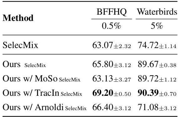
This table presents the average accuracy and standard error for different bias mitigation methods across various datasets (CMNIST, CIFAR10C, BFFHQ) and bias levels (0.5%, 1%, 2%, 5%). It compares the performance of several existing methods (ERM, LfF, DFA, SelecMix) with and without the proposed method, denoted as ‘Ours’. The ‘Info’ column indicates whether the method utilizes bias information or not. Bold values highlight the best-performing method for each dataset and bias level.

This table presents the average accuracy and standard error, over three runs, for different bias mitigation methods across four datasets (CMNIST, CIFAR10C, BFFHQ, Waterbirds) and varying bias ratios (0.5%, 1%, 2%, 5%). The ‘Ours’ methods show the performance of the proposed method when applied to models pre-trained with other methods (ERM, LfF, DFA, SelecMix). The best accuracy for each condition is highlighted in bold. The table also indicates whether each method utilizes bias information (✓) or not (X).
Full paper#


