↗ OpenReview ↗ NeurIPS Homepage ↗ Chat
TL;DR#
Estimating conditional probability distributions is crucial for various machine learning tasks, including risk assessment and uncertainty quantification. However, existing methods face challenges such as computational inefficiency, retraining needs, and a lack of theoretical guarantees. These methods also struggle with high-dimensional data and complex distributions.
This paper introduces Neural Conditional Probability (NCP), a novel approach that addresses these limitations. NCP leverages the power of neural networks to learn the conditional expectation operator, allowing efficient computation of various statistics without retraining. The method is supported by theoretical guarantees ensuring both optimization consistency and statistical accuracy. Experimental results on various datasets demonstrate NCP’s competitive performance, even compared to more complex models.
Key Takeaways#
Why does it matter?#
This paper is important because it presents a novel and efficient approach to learning conditional probability distributions, a fundamental problem in many machine learning applications. The theoretical guarantees and experimental results demonstrate its effectiveness, making it relevant to researchers working on various applications involving uncertainty quantification. The proposed method opens new avenues for research by enabling more streamlined inference and providing theoretical guarantees, which were lacking in existing methods.
Visual Insights#

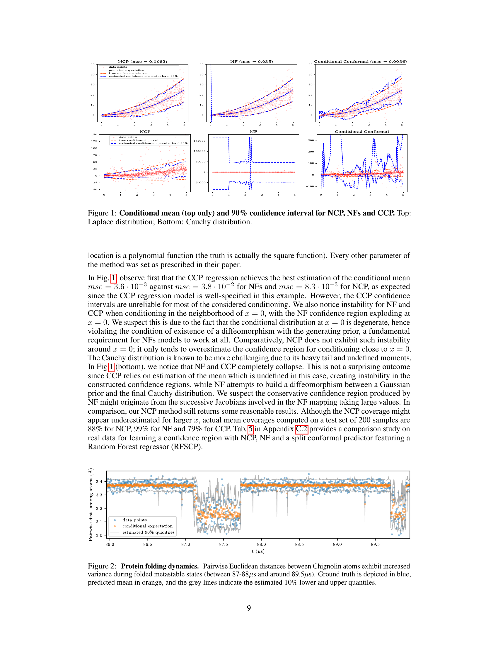
This figure compares the performance of three methods – NCP, Normalizing Flows (NF), and Conditional Conformal Prediction (CCP) – in estimating the conditional mean and 90% confidence intervals for two different distributions: Laplace (top) and Cauchy (bottom). For each distribution, the figure shows the true conditional mean (orange dashed line), the estimated conditional mean from each method (solid lines), the true 90% confidence interval (blue dashed lines), and the 90% confidence interval estimated by each method (blue solid lines). The plots demonstrate the effectiveness of NCP in producing accurate estimates and reliable confidence intervals, particularly when compared to NF and CCP which show instability and less accurate estimation in certain areas..
This table presents the results of a comparison study between eleven different methods for conditional density estimation. The performance metric used is the Kolmogorov-Smirnov (KS) distance between the estimated and true conditional cumulative distribution functions (CDFs). The mean and standard deviation of the KS distance are reported for each method, averaged over ten repetitions, each with a different random seed. The best-performing method for each dataset is highlighted in red, while the second-best method is shown in bold black.
In-depth insights#
Conditional Density#
Conditional density estimation is a crucial problem in various fields, aiming to model the probability distribution of a variable given the value of another. The challenge lies in accurately capturing the complex relationships between variables, especially in high-dimensional settings. Non-parametric methods, while flexible, often suffer from the curse of dimensionality. Parametric approaches, such as Gaussian mixture models, offer computational efficiency but may not accurately represent complex distributions. Recent advances leverage deep learning, utilizing neural networks to learn flexible and high-dimensional conditional densities. However, such approaches often require significant data and computational resources, potentially raising concerns about scalability and reproducibility. Operator-theoretic methods provide a promising alternative by directly learning the conditional expectation operator, offering efficient inference and theoretical guarantees. This approach requires a careful selection of the loss function and network architecture to balance accuracy and efficiency. Careful consideration of the model’s limitations and assumptions, such as the required sample size and the impact of high dimensionality, is crucial for reliable results and responsible deployment.
Operator Approach#
The ‘Operator Approach’ section of this PDF likely details a novel method for learning conditional probability distributions. Instead of directly modeling the conditional density, it leverages the theory of conditional expectation operators. This involves framing the problem within a functional analysis setting, where the conditional expectation is treated as an operator mapping functions of one variable to functions of another. This approach offers several potential advantages. First, it allows for the estimation of various conditional statistics (mean, variance, quantiles) from a single, trained operator, rather than requiring separate models for each statistic. Second, it may offer greater efficiency and scalability, particularly in high-dimensional settings where traditional density estimation methods struggle. Theoretical guarantees on the accuracy of the resulting estimates are likely provided, along with details on the loss functions used for training the operator. This framework likely uses neural networks to approximate the operator, offering a principled way to combine the strengths of operator theory and machine learning for complex probabilistic inference tasks. The core innovation might lie in the specific loss function used to optimize the neural network approximation of the operator. This loss function likely guarantees both the optimization’s consistency and the statistical accuracy of the learned model.
NCP Architecture#
The Neural Conditional Probability (NCP) architecture, while not explicitly detailed as a separate heading, is implicitly defined by the paper’s description of its components and training process. The core of the NCP architecture centers around using neural networks to parameterize the singular value decomposition (SVD) of the conditional expectation operator. This involves two embedding networks, uθ(x) and vθ(y), which map the input variables X and Y into a shared latent space of dimension d. A third network parameterizes the singular values, σθ, which are usually implemented as positive values. The choice of network architecture, such as the depth and width of the hidden layers and activation functions, directly affects the model’s capacity and performance. The training of the NCP model aims to optimize a loss function that encourages both accurate representation of the joint distribution in the latent space and the alignment of latent space metrics with those of the input variables, ensuring good generalization performance. The described training procedure uses a two-hidden layer MLP architecture; however, the paper suggests that the choice of architecture is flexible and can be adapted to specific needs. The architecture’s simplicity contrasts with the complex nature of the problems it tackles, thus highlighting the effectiveness of the theoretically grounded loss function used in training.
Learning Guarantees#
The section on ‘Learning Guarantees’ in a machine learning research paper is crucial for establishing the reliability and trustworthiness of the proposed model. It delves into the theoretical analysis, providing mathematical proofs and bounds to ensure the model’s performance converges to the true underlying distribution. This section should rigorously demonstrate consistency (does the model learn the correct function as the training data grows?), generalization ability (how well does the model perform on unseen data?), and convergence rates (how quickly does the model improve with more data?). Specific theorems and lemmas rigorously formalize these properties, highlighting assumptions made about the data distribution and model architecture. The success of these proofs directly impacts the confidence in the model’s results; robust learning guarantees provide reassurance, while weak guarantees raise concerns about the model’s dependability and potential overfitting. This section might also address the impact of hyperparameters on generalization and provide bounds on error metrics to gauge the model’s performance within specific conditions. Overall, the quality and comprehensiveness of the Learning Guarantees section significantly contribute to the paper’s credibility and scientific value.
Future Research#
The paper’s core contribution is a novel method for learning conditional probability distributions, demonstrating strong performance and theoretical grounding. Future research could focus on several key areas. First, extending the methodology to handle more complex data structures such as time series or graphs would significantly expand its applicability. Second, exploring more sophisticated neural network architectures beyond the minimalistic two-hidden-layer network used in the paper could potentially boost performance, especially on high-dimensional datasets. Third, developing more efficient training algorithms and optimization strategies is crucial for scaling to even larger datasets. Finally, a deep dive into the practical implications and applications of the method across various domains is needed to truly showcase its potential and address specific challenges in those fields. The exploration of these avenues would not only strengthen the theoretical framework but also demonstrate the practical impact of this innovative methodology.
More visual insights#
More on figures

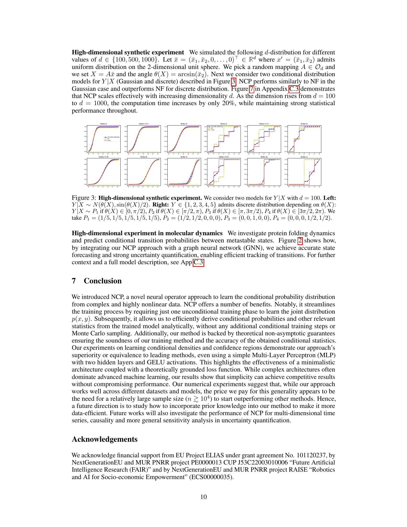
This figure shows the results of applying the NCP method to predict the pairwise Euclidean distances between atoms in a protein (Chignolin) during a folding simulation. The x-axis represents time (in microseconds), and the y-axis represents the pairwise distance. The blue dots show the actual data points from the simulation. The orange line shows the conditional expectation of the distance predicted by the NCP model at each time point, and the grey lines indicate the 10% lower and upper quantiles. The figure highlights that the NCP model successfully predicts not only the mean distance but also its uncertainty.

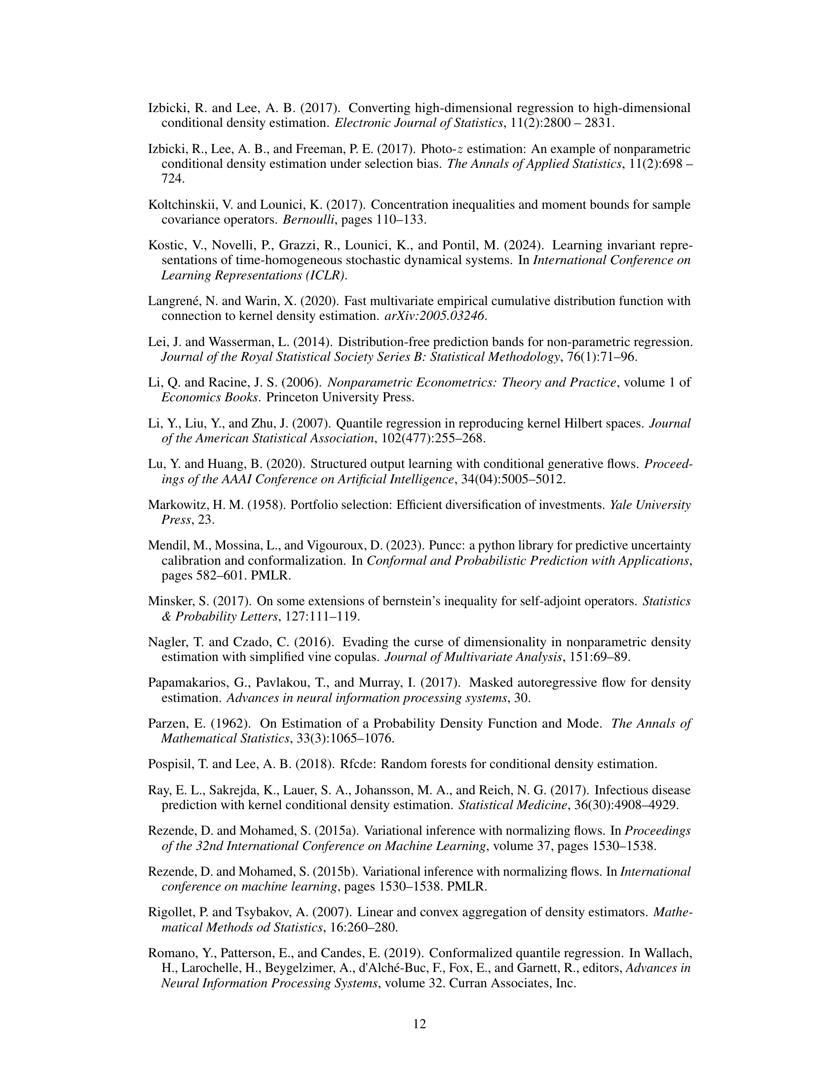
This figure shows the results of a high-dimensional synthetic experiment to evaluate the performance of the NCP model in estimating conditional distributions. Two models for Y|X were considered with dimension d=100: a Gaussian model and a discrete model. The Gaussian model’s parameters depend on the angle θ(X), and its distribution is normal with mean θ(X) and standard deviation sin(θ(X)/2). The discrete model’s distribution depends on the range of θ(X), assigning different probability distributions (P₁, P₂, P₃, P₄) to different ranges of θ(X). The results shown in the figure’s plots illustrates the performance of NCP under these different model conditions.

This figure shows the training and validation loss curves for a Laplace experiment described in Section 6 of the paper. The x-axis represents the number of epochs (iterations) during training, and the y-axis represents the value of the loss function. The plot illustrates how the loss decreases over time for both the training and validation datasets, indicating the model’s learning progress. The relatively close proximity of the training and validation loss curves suggests that the model is not overfitting significantly.
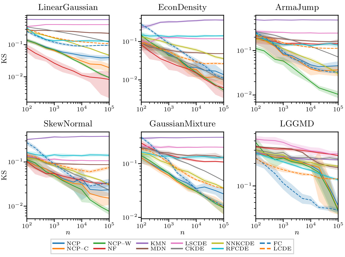
This figure displays the performance of different conditional density estimation (CDE) methods across six synthetic datasets with varying sample sizes (n). The x-axis represents the sample size (n), and the y-axis represents the Kolmogorov-Smirnov (KS) distance, which measures the difference between the estimated and true cumulative distribution functions (CDFs). Lower KS distance indicates better performance. The figure shows that the performance of most methods improves with increasing sample size. The NCP methods (NCP, NCP-C, and NCP-W) generally show competitive or better performance compared to other methods.
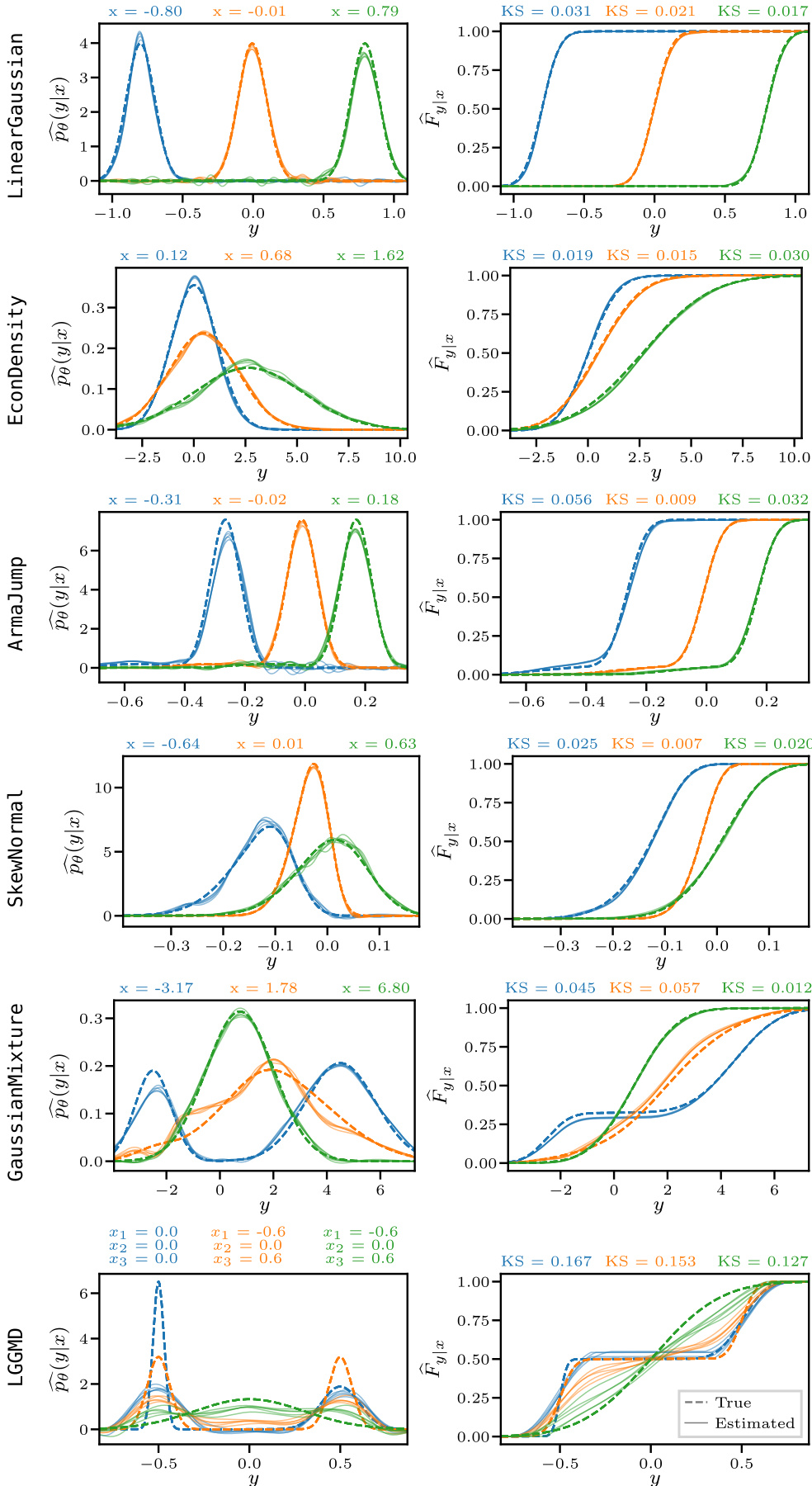
This figure compares the estimated and true probability density functions (PDFs) and cumulative distribution functions (CDFs) for six synthetic datasets. Three different conditioning points are shown for each dataset. The left column displays the PDFs, and the right column displays the CDFs. Dotted lines represent the true distributions, and solid lines show the estimates generated by the Neural Conditional Probability (NCP) method. The Kolmogorov-Smirnov (KS) statistic, a measure of the distance between the estimated and true CDFs, is provided for each conditioning point, quantifying the accuracy of the NCP estimations.
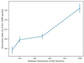
This figure shows the scalability of NCP with respect to increasing dimensionality. The left panel shows that the computation time only increases by about 20% when the dimension increases from 100 to 1000. The right panel shows the average Kolmogorov-Smirnov (KS) distance between the estimated and true conditional CDFs for different dimensions, demonstrating that NCP maintains strong statistical performance even in high-dimensional settings.
More on tables
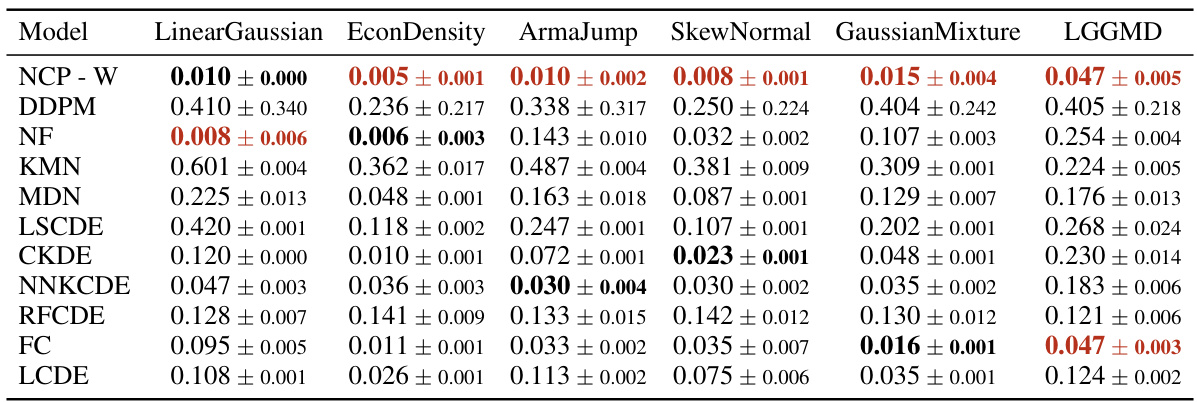
This table presents the performance comparison of several conditional density estimation methods. The Kolmogorov-Smirnov (KS) distance, a metric measuring the difference between two cumulative distribution functions (CDFs), was used to assess the accuracy of the estimated conditional CDFs against the true conditional CDFs. The experiment was conducted 10 times with a sample size of 105, and the mean and standard deviation of the KS distance are reported. The best-performing method for each dataset is highlighted in red, while the second-best is shown in bold black.
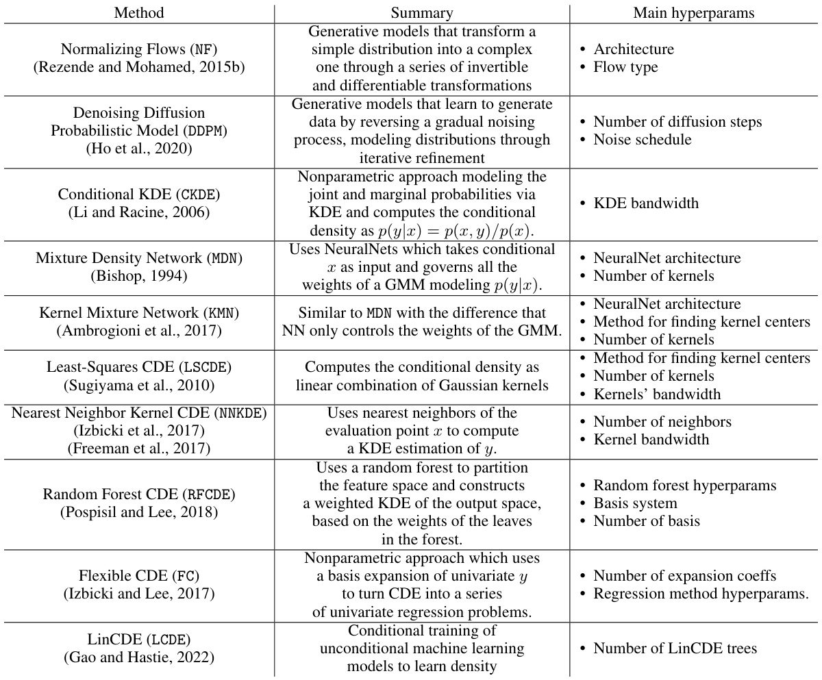
This table presents the results of comparing the performance of different conditional density estimation methods. The Kolmogorov-Smirnov (KS) distance, a metric that measures the difference between two cumulative distribution functions (CDFs), is used to evaluate how well each method estimates the true conditional CDF. The mean and standard deviation of the KS distance are reported, calculated across 10 repetitions of the experiment, each with a different random seed. The best and second-best performing methods for each dataset are highlighted in red and bold black, respectively. The sample size (n) used for the experiments is 105.

This table presents the performance comparison of different conditional density estimation methods. The Kolmogorov-Smirnov (KS) distance, a metric measuring the difference between two cumulative distribution functions, is used to evaluate the accuracy of each method in estimating the conditional cumulative distribution function (CDF). The results are averaged over 10 repetitions, each with a different random seed, for a sample size of n=105. The best-performing method for each dataset is highlighted in red, while the second-best is shown in bold black.

This table presents the results of comparing different methods for estimating conditional cumulative distribution functions (CDFs). The Kolmogorov-Smirnov (KS) distance, a metric measuring the difference between two CDFs, was calculated for each method across ten repetitions, using a sample size of 105. The best-performing method for each dataset is highlighted in red, while the second-best is shown in bold black. The results provide a quantitative comparison of the accuracy of various approaches.
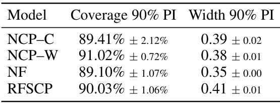
This table presents the results of a comparison of different methods for conditional density estimation. The performance metric is the Kolmogorov-Smirnov (KS) distance between the estimated and true cumulative distribution functions (CDFs). The mean and standard deviation of the KS distance are reported, averaged over 10 repetitions, each using a different random seed and a sample size of n=105. The best-performing method for each dataset is highlighted in red, and the second-best is in bold black.

This table presents the results of the conditional density estimation experiments. It shows the Kolmogorov-Smirnov (KS) distance between the estimated cumulative distribution function (CDF) and the true CDF for various models. The results are averaged over 10 repetitions with a sample size of 105. The best performing model for each dataset is highlighted in red, while the second-best is shown in bold black. The table allows for comparison of the accuracy of different conditional density estimation methods.
Full paper#

