↗ OpenReview ↗ NeurIPS Proc. ↗ Chat
TL;DR#
Estimating the Lipschitz constant of deep neural networks is crucial for verifying their robustness but computationally expensive using existing methods. These existing methods often involve solving large-scale matrix verification problems, hindering their applicability to larger and deeper networks. This poses a significant challenge for certifying the robustness of increasingly complex models.
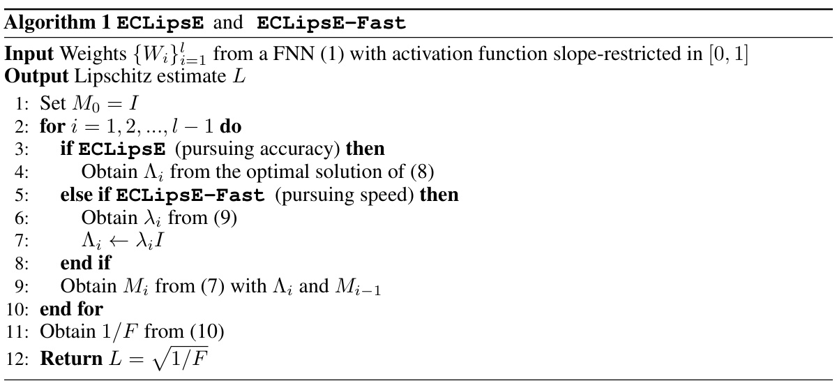
The paper introduces ECLipsE, a compositional approach to efficiently estimate Lipschitz constants. It leverages a sequential Cholesky decomposition to break down the large problem into smaller subproblems. Two algorithms are developed: ECLipsE solves small semidefinite programs, while ECLipsE-Fast provides a closed-form solution for extremely fast estimation. Experiments demonstrate significant speedups (up to several thousand times) over state-of-the-art methods, while achieving similar or even better accuracy in Lipschitz bound estimation.
Key Takeaways#
Why does it matter?#
This paper is crucial for researchers working on neural network robustness certification because it introduces a highly efficient and scalable method for estimating Lipschitz constants. This is a significant advancement in the field, enabling the verification of neural networks with greater depth and width than previously possible. The work opens avenues for further research into compositional approaches, improving the scalability and efficiency of existing certification techniques, and extending these methods to other neural network architectures such as CNNs and Residual Networks.
Visual Insights#

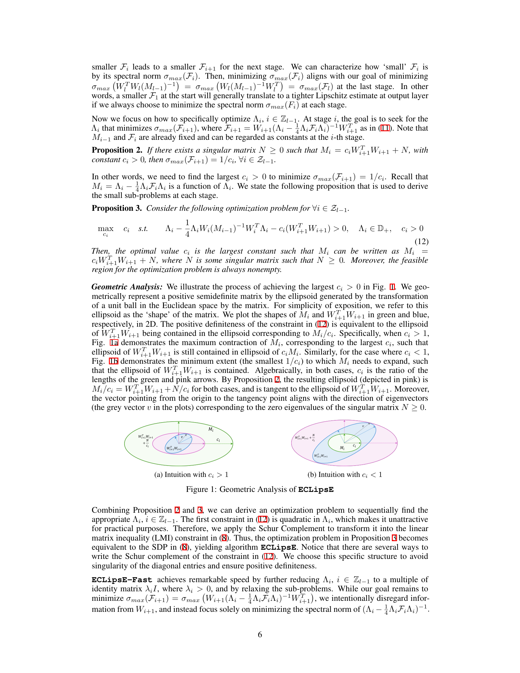
This figure geometrically illustrates the process of finding the largest constant ci in the optimization problem (12) for algorithm ECLipsE. It uses ellipsoids to represent positive semidefinite matrices. The green ellipsoid represents Mi, the blue ellipsoid represents Wi+1WTi+1, and the pink ellipsoid represents Mi/ci. Panel (a) shows the case where ci > 1, illustrating how the ellipsoid of Wi+1WTi+1 is contained within the contracted ellipsoid Mi/ci. Panel (b) shows the case where ci < 1, illustrating how the ellipsoid Mi needs to expand to contain Wi+1WTi+1. The grey vector v points to the direction of the zero eigenvector of the singular matrix N. The figure visually demonstrates the relationship between the matrix inequalities, the geometric interpretation of the solution, and how finding the optimal ci leads to a tighter Lipschitz estimate.
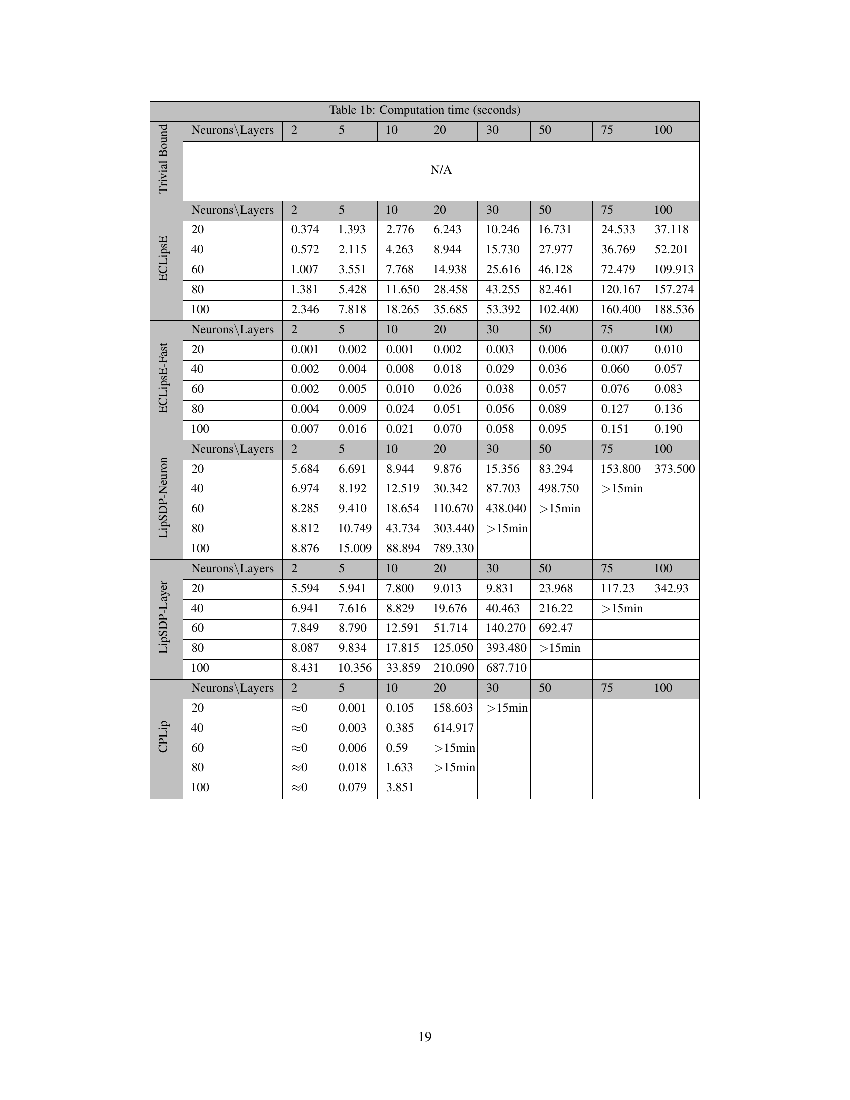
This table presents the computation time, in seconds, required for various algorithms (ECLipsE, ECLipsE-Fast, LipSDP-Neuron, LipSDP-Layer, and CPLip) to estimate the Lipschitz constant for randomly generated neural networks with varying numbers of neurons and layers. The table showcases the significant speed advantage of ECLipsE and especially ECLipsE-Fast, particularly as network size increases.
In-depth insights#
LipConst Estimation#
Estimating Lipschitz constants for neural networks (LipConst Estimation) is crucial for verifying their robustness. The challenge lies in the computational complexity, especially for deep networks. This paper proposes a compositional approach, breaking down the problem into smaller, layer-wise subproblems. Two algorithms are presented: ECLipsE, which solves small semidefinite programs (SDPs), and ECLipsE-Fast, offering closed-form solutions for significantly faster computation. While ECLipsE prioritizes accuracy, ECLipsE-Fast excels in speed, achieving up to thousands of times faster computation compared to state-of-the-art methods. The core innovation is a novel decomposition technique and a geometrical analysis supporting these algorithms’ accuracy and efficiency. Experimental results across various network architectures confirm the dramatic speedup without compromising accuracy significantly, enhancing the feasibility of robustness certification in real-world applications.
Compositional Algo#
The heading ‘Compositional Algo’ likely refers to a section detailing algorithms designed for compositional estimation of Lipschitz constants. This approach is crucial because directly computing Lipschitz constants for deep neural networks is computationally expensive. A compositional method breaks down the complex problem into smaller, manageable subproblems, one for each layer. This significantly reduces computational cost, especially for deep networks. The algorithms likely leverage the layered structure of neural networks, processing each layer’s contribution independently before combining the results. Two algorithms are suggested, possibly representing a tradeoff between speed and accuracy. One might be a more precise approach involving semidefinite programming (SDP) solutions on smaller matrices per layer, while the other prioritizes speed through a closed-form solution, potentially at the cost of some accuracy. The effectiveness of these compositional algorithms is likely demonstrated empirically by showing their superior runtime performance compared to traditional methods, while achieving comparable or even better accuracy in estimating Lipschitz bounds. The core innovation is in the clever decomposition of the problem, enabling scalable and efficient certification of neural network robustness.
Scalability & Speed#
The research paper emphasizes scalability and speed as crucial aspects of its proposed compositional approach for Lipschitz constant estimation. Existing methods often struggle with the computational cost associated with high-dimensional data and deep networks. The authors’ compositional algorithms, ECLipsE and ECLipsE-Fast, address these limitations by decomposing the large optimization problem into smaller, more manageable subproblems solved layer-by-layer. This decomposition allows for significant computational speedups (thousands of times faster than state-of-the-art methods), which is particularly critical for online learning applications. ECLipsE-Fast, leveraging closed-form solutions, achieves the highest speed at the cost of slightly reduced accuracy, while ECLipsE maintains higher accuracy at a moderate speed improvement. The paper demonstrates the efficiency of its approach through extensive experiments on randomly generated networks and those trained on MNIST, showcasing scalability to significantly deeper and wider networks than previously possible. Improved scalability and reduced computation time makes the method very attractive for applications that demand real-time or near real-time analysis.
Geometric Analysis#
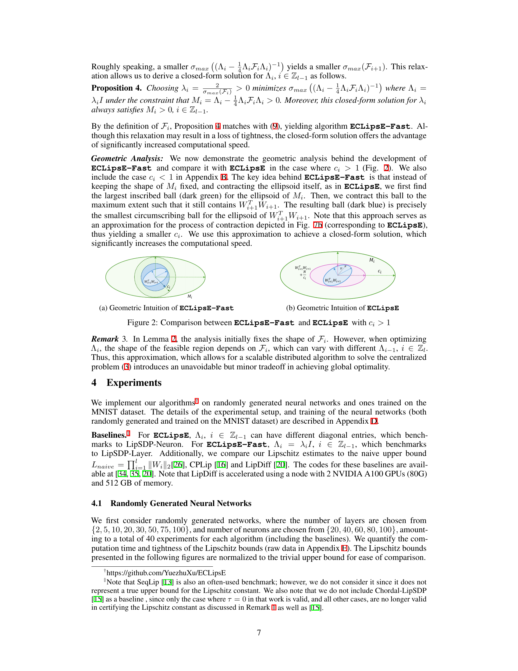
The “Geometric Analysis” section likely provides a visual and intuitive explanation of the algorithms’ optimization strategies. It probably uses geometric concepts, such as ellipsoids, to represent matrices and illustrate how the algorithms iteratively refine Lipschitz constant estimates. The authors might visually depict the contraction or expansion of these shapes to show how the algorithms minimize the spectral norm of specific matrices, ultimately leading to a tight Lipschitz bound. Key visualizations might include comparisons between different algorithms, highlighting how their geometric approaches differ in efficiency and accuracy. The analysis likely supports the theoretical claims, providing a compelling visual aid to the reader for better comprehension of the complex mathematical operations. A crucial aspect of this section could be showing how geometric properties of the optimization problems (such as the feasible region) are exploited by the algorithms, suggesting the strong relationship between the geometric interpretation and algorithmic design.
Future Research#
The “Future Research” section of this paper could explore several promising avenues. Extending the compositional approach to other network architectures, such as convolutional neural networks (CNNs) and recurrent neural networks (RNNs), is crucial. Current methods often struggle with these complex structures, demanding novel decompositions and efficient algorithms. Improving the scalability of the algorithms for extremely large networks is another key area. The paper acknowledges that computational costs can increase significantly with wider networks; addressing this through advanced optimization or approximation techniques could broaden the applicability of the approach. Investigating the trade-offs between accuracy and efficiency more thoroughly is warranted. While two algorithms are presented, a deeper analysis comparing their performance under various conditions and potential hybrid approaches would enhance the understanding of this trade-off. Finally, exploring the potential applications of the proposed compositional approach in other domains like reinforcement learning, control systems, and online learning is highly important, demonstrating the wider implications of robust Lipschitz constant estimation.
More visual insights#
More on figures
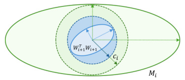
This figure provides a geometric interpretation of the optimization problem in Proposition 3. It illustrates how the largest constant (c_i) can be found by comparing the shapes of matrices (M_i) and (W_{i+1}W_{i+1}^T), represented as ellipsoids. The green ellipsoid represents (M_i), and the blue ellipsoid represents (W_{i+1}W_{i+1}^T). The pink ellipsoid shows the result of the contraction, where (c_i) represents the ratio between the lengths of the green and pink arrows. Figure (a) demonstrates the case where (c_i > 1), while Figure (b) shows (c_i < 1).
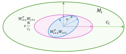
This figure geometrically illustrates the process of finding the optimal value of (c_i) in the optimization problem (12). It uses ellipsoids to represent positive semidefinite matrices. The blue ellipsoid represents (W_{i+1}W_{i+1}^T), the green ellipsoid depicts (M_i), and the pink ellipsoid shows (M_i/c_i). The figure demonstrates how, by adjusting (c_i), the ellipsoid (W_{i+1}W_{i+1}^T) can be contained within (M_i/c_i). The optimal (c_i) is the largest value that allows this containment while ensuring (M_i > 0). (a) shows the case where (c_i > 1), representing a contraction of the ellipsoid, and (b) illustrates the case where (c_i < 1), indicating an expansion of the ellipsoid.
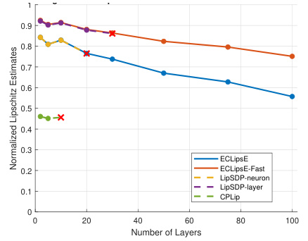
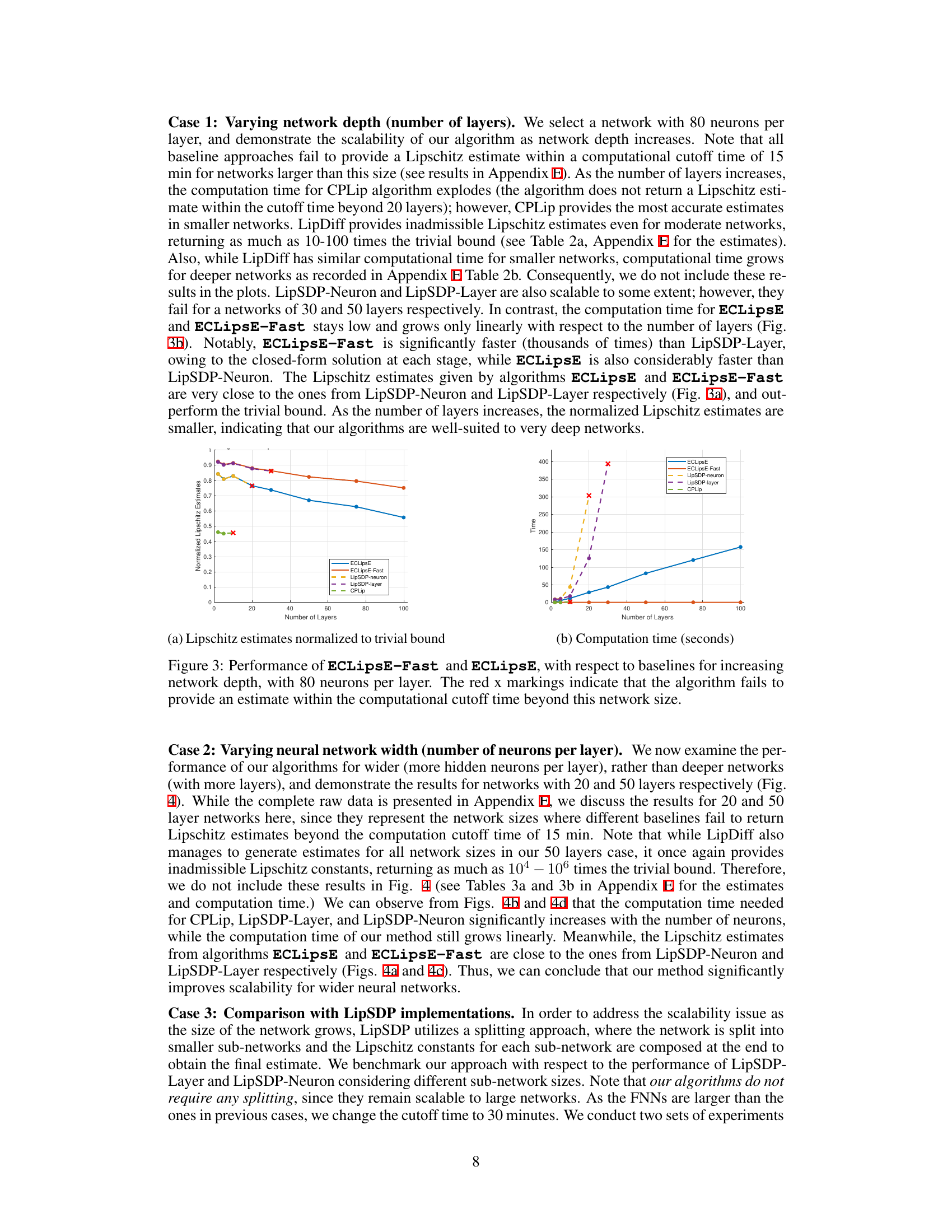
This figure compares the performance of ECLipsE and ECLipsE-Fast algorithms against several baseline methods (LipSDP-neuron, LipSDP-layer, and CPLip) for estimating the Lipschitz constant of neural networks with varying depths (number of layers). The x-axis represents the number of layers, while the y-axis represents the normalized Lipschitz estimates. The plot shows that both ECLipsE and ECLipsE-Fast maintain efficiency and accuracy with increasing network depth, while baseline methods struggle and fail to provide estimates beyond a certain number of layers (indicated by red ‘x’ marks).
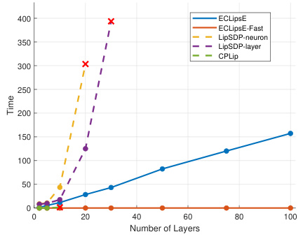
The figure shows the performance comparison of ECLipsE and ECLipsE-Fast algorithms against baseline methods (LipSDP-neuron, LipSDP-layer, and CPLip) for estimating Lipschitz constants of neural networks with varying depth (number of layers). The x-axis represents the number of layers, and the y-axis represents the computation time in seconds. ECLipsE-Fast shows significantly faster computation times compared to all other algorithms, especially as the network depth increases. ECLipsE also shows a considerable speed advantage over LipSDP algorithms. The red ‘x’ markers highlight where the baseline algorithms failed to provide estimates within the given time limit.
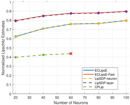
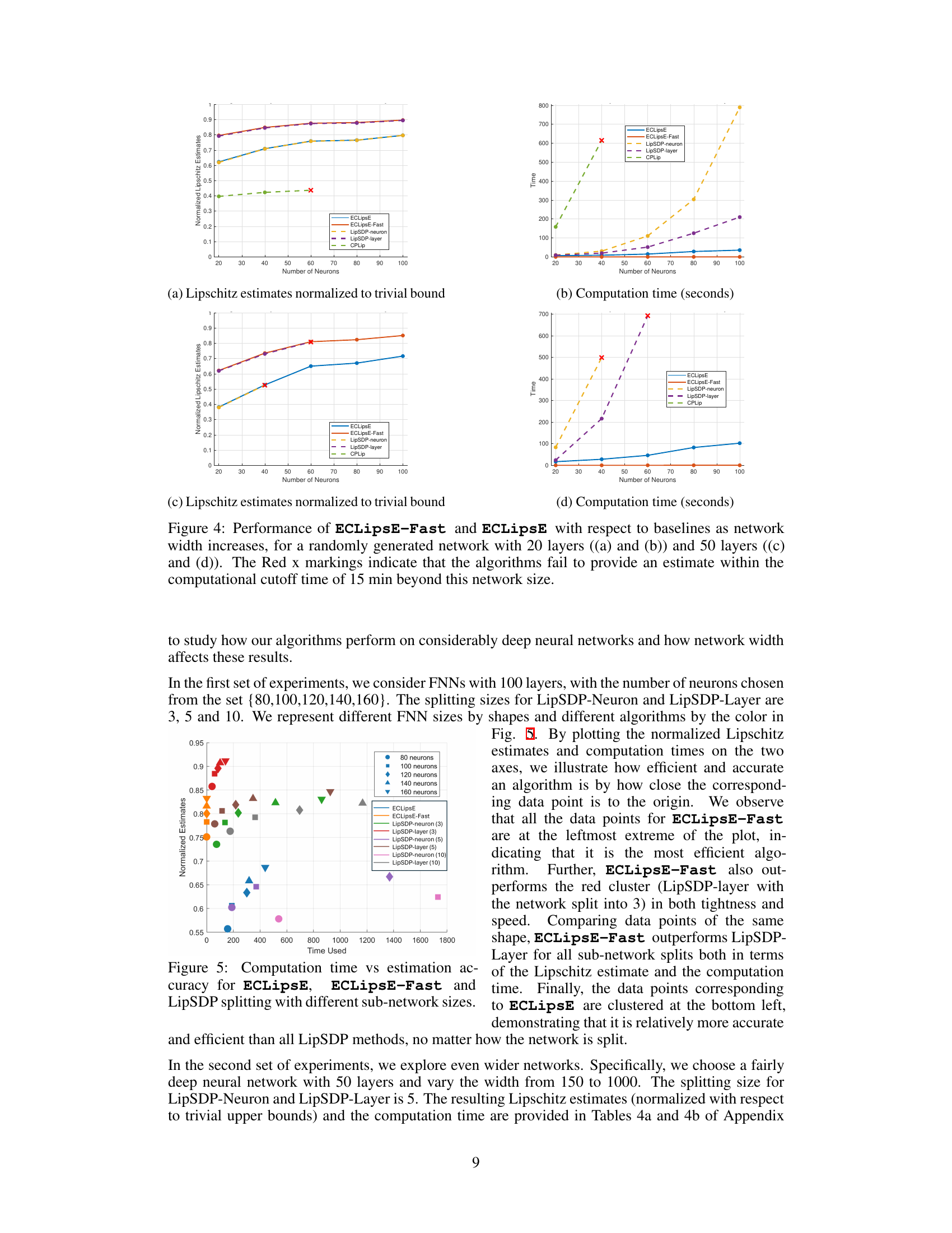
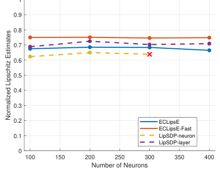
This figure compares the performance of ECLipsE and ECLipsE-Fast against various baseline methods (LipSDP-neuron, LipSDP-layer, CPLip) as the width (number of neurons per layer) of randomly generated neural networks increases. Two network depths are shown: 20 layers and 50 layers. The plots show normalized Lipschitz estimates and computation times. The red ‘x’ denotes cases where the baseline methods failed to produce results within the 15-minute time limit. The results illustrate the scalability and efficiency of the proposed ECLipsE algorithms, particularly ECLipsE-Fast, even with wider networks.
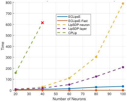
This figure demonstrates the scalability of ECLipsE and ECLipsE-Fast algorithms in comparison with other baseline methods such as LipSDP-Neuron, LipSDP-Layer and CPLip, as the width of the network (number of neurons per layer) increases. Subfigures (a) and (c) show the normalized Lipschitz estimates while (b) and (d) show the computation time. The results show that ECLipsE and ECLipsE-Fast maintain good scalability and accuracy even as the network becomes wider, while other methods fail to produce estimates within a 15-minute time limit for wider networks.
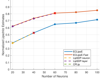
This figure shows the performance comparison of ECLipsE and ECLipsE-Fast algorithms against several baseline methods (LipSDP-neuron, LipSDP-layer, CPLip) for randomly generated neural networks. The comparison is made by varying the number of neurons (network width) while keeping the number of layers fixed at 20 and 50. The plots show both normalized Lipschitz estimates and computation time in seconds. The red ‘x’ marks indicate cases where baseline algorithms failed to provide estimates within the 15-minute time limit.
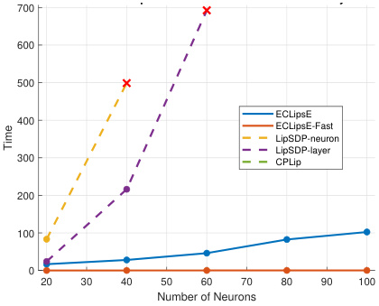
This figure demonstrates the scalability and efficiency of the proposed algorithms (ECLipsE and ECLipsE-Fast) compared to baseline methods (LipSDP-neuron, LipSDP-layer, and CPLip) as the width (number of neurons per layer) of randomly generated neural networks increases. It shows the normalized Lipschitz estimates and computation times for networks with 20 and 50 layers. The results highlight that ECLipsE and ECLipsE-Fast maintain relatively low computation times even with increasing network width, unlike the baseline methods which struggle to provide estimates within the time limit for wider networks.
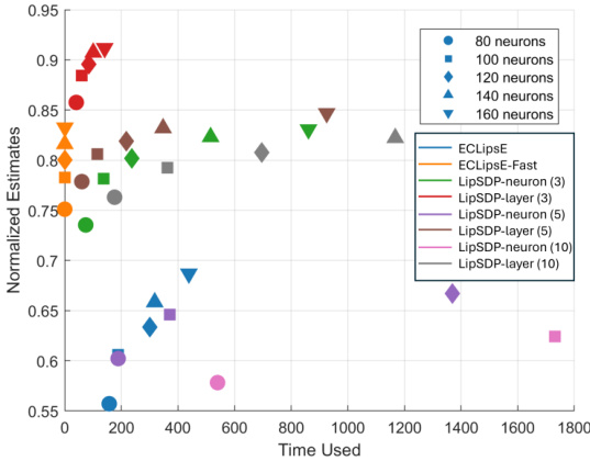
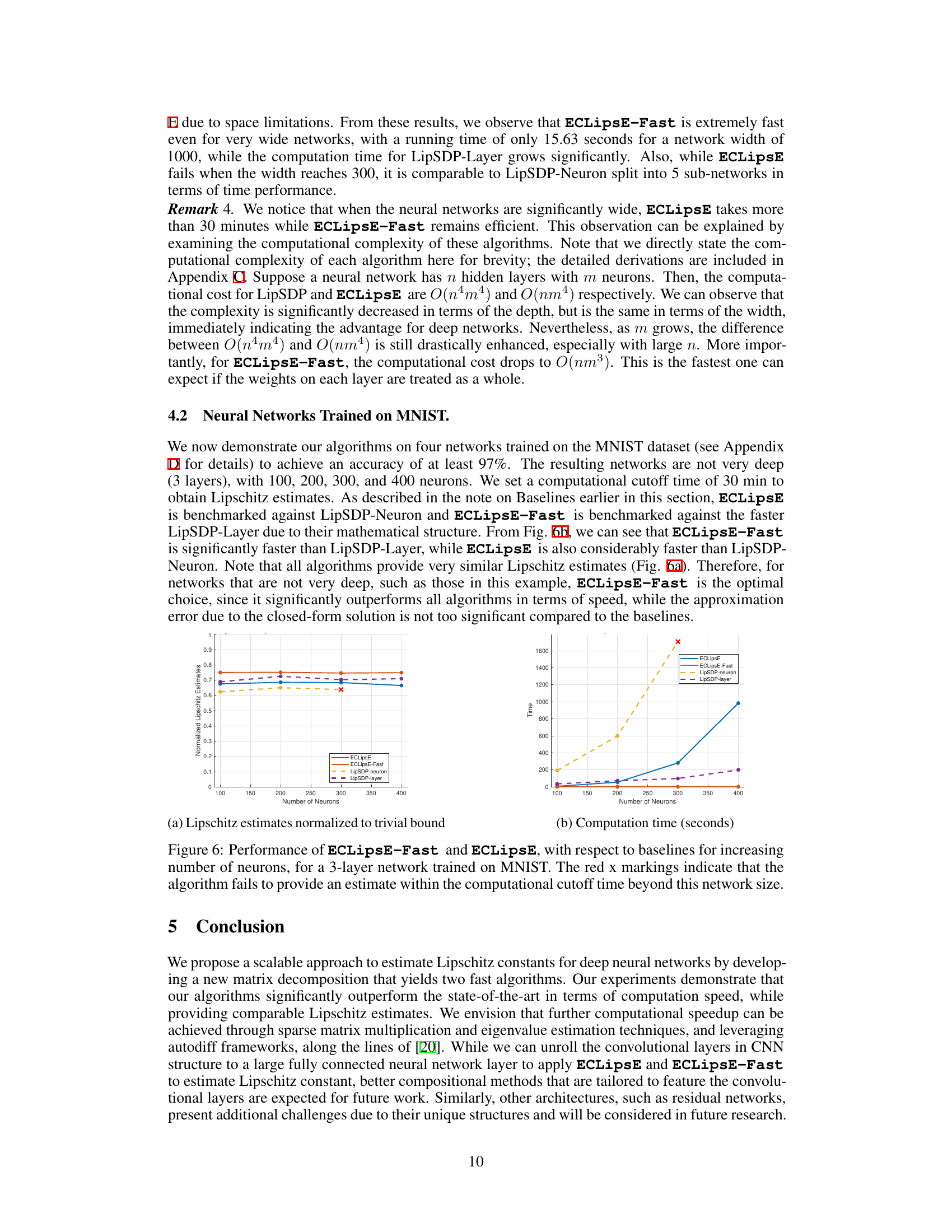
This figure compares the computation time and estimation accuracy of ECLipsE, ECLipsE-Fast, and LipSDP (with different sub-network splitting sizes) for neural networks with 100 layers and varying neuron counts (80, 100, 120, 140, 160). The x-axis represents the computation time used, and the y-axis represents the normalized Lipschitz estimates. The plot shows that ECLipsE-Fast consistently achieves the lowest computation times, while maintaining relatively high accuracy. ECLipsE also demonstrates good efficiency and accuracy, outperforming LipSDP across different splitting sizes.
This figure compares the performance of the proposed algorithms, ECLipsE and ECLipsE-Fast, against several baseline methods (LipSDP-neuron, LipSDP-layer, and CPLip) for estimating the Lipschitz constant of neural networks with varying depth. The x-axis represents the number of layers, while the y-axis shows the normalized Lipschitz estimates and the computation time (in seconds). The plot highlights that ECLipsE and ECLipsE-Fast are scalable to much deeper networks compared to the baselines, which fail to provide estimates beyond a certain depth (indicated by red ‘x’ marks). Notably, ECLipsE-Fast is significantly faster than others while maintaining accuracy.
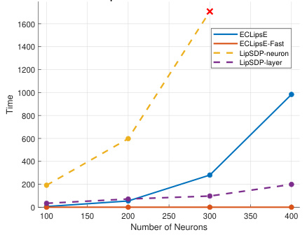
This figure compares the performance of ECLipsE and ECLipsE-Fast against baseline methods (CPLip, LipSDP-neuron, LipSDP-layer, and LipDiff) as the width (number of neurons per layer) of randomly generated neural networks increases. The networks have 20 and 50 layers. The plots show (a,c) normalized Lipschitz estimates and (b,d) computation times (in seconds). The red ‘x’ symbol indicates that a method failed to return an estimate within the 15-minute time limit.

This figure provides a geometric interpretation of the optimization problem in Proposition 3. Panel (a) illustrates the case where the optimal value (c_i > 1), showing how the ellipsoid representing (M_i) contracts to contain the ellipsoid representing (W_{i+1}W_{i+1}^T). The largest such contraction is shown to be tangent to (W_{i+1}W_{i+1}^T). Panel (b) shows the case where (c_i < 1), illustrating the expansion needed for (M_i) to contain (W_{i+1}W_{i+1}^T). In both cases, the relationship between the ellipsoids demonstrates the geometric meaning of maximizing (c_i).
More on tables
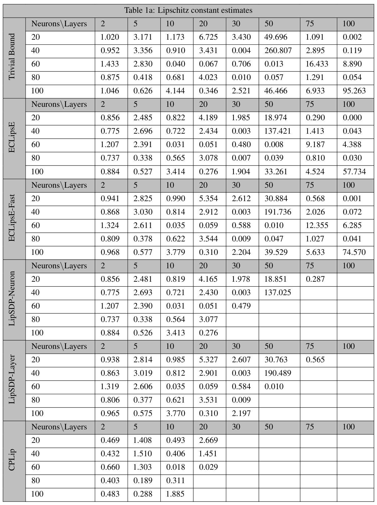
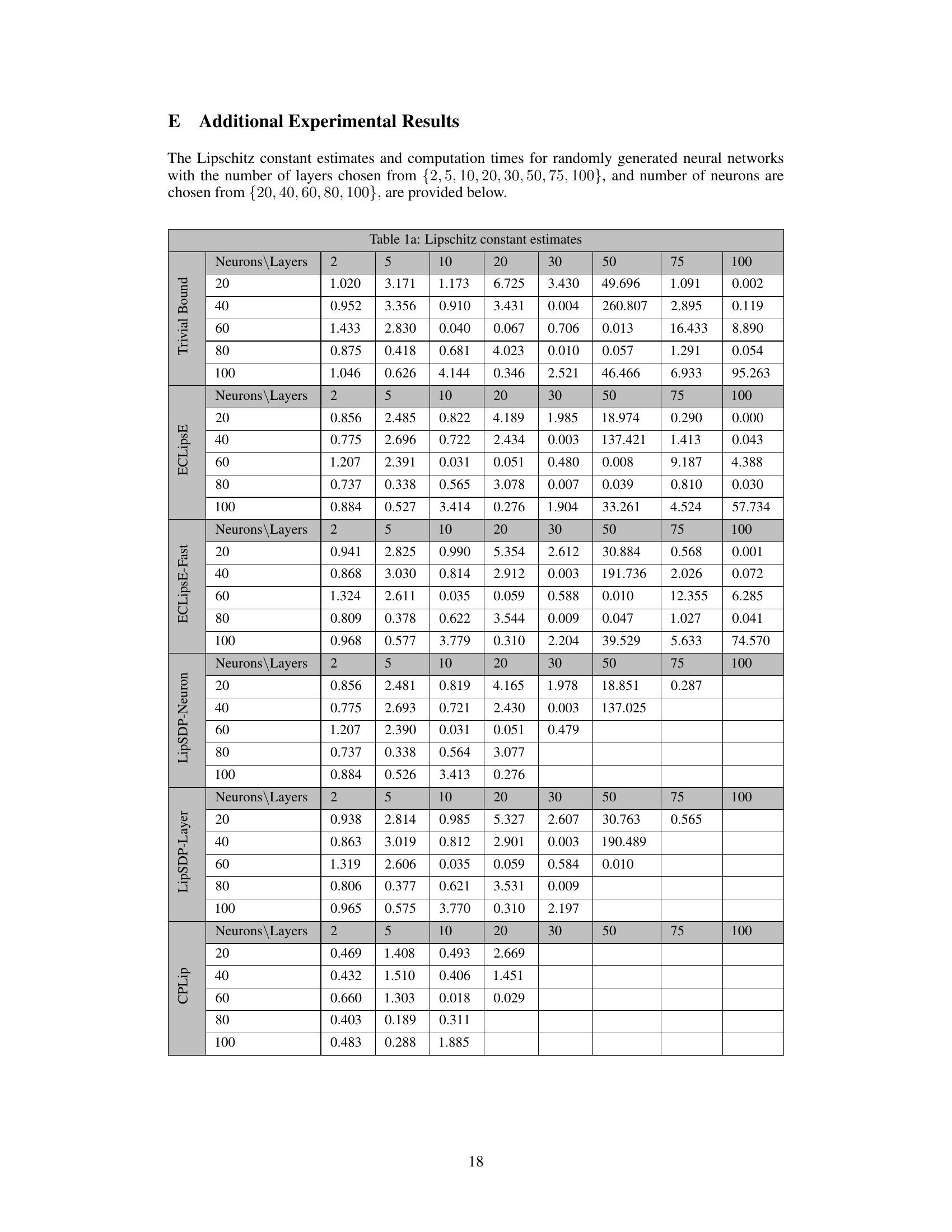
This table presents the Lipschitz constant estimates obtained using different methods (ECLipsE, ECLipsE-Fast, LipSDP-Neuron, LipSDP-Layer, and CPLip) for randomly generated neural networks with varying numbers of neurons (20, 40, 60, 80, 100) and layers (2, 5, 10, 20, 30, 50, 75, 100). The ‘Trivial Bound’ column provides a naive upper bound for comparison. The table demonstrates the accuracy and scalability of the proposed methods.
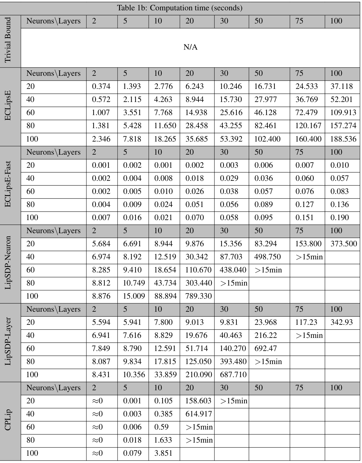
This table presents the computation time in seconds for randomly generated neural networks with varying numbers of neurons (20, 40, 60, 80, 100) and layers (2, 5, 10, 20, 30, 50, 75, 100). The algorithms compared include ECLipSE, ECLipSE-Fast, LipSDP-Neuron, LipSDP-Layer, and CPLip. The table shows how the computation time increases with the number of neurons and layers for each algorithm, highlighting the scalability and efficiency differences among the methods. Note that LipSDP-Neuron and LipSDP-Layer fail to provide results for larger networks within the 15-minute time limit.

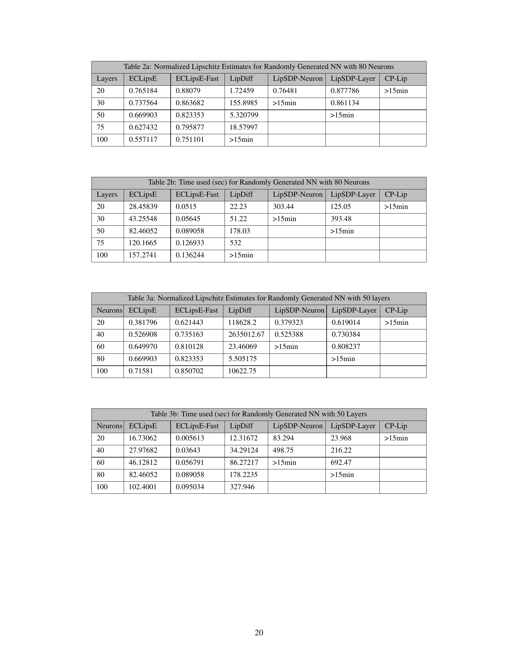
This table presents the normalized Lipschitz constant estimates obtained using various methods (ECLipsE, ECLipsE-Fast, LipDiff, LipSDP-Neuron, LipSDP-Layer, and CP-Lip) for randomly generated neural networks with 80 neurons per layer and varying depths (number of layers). The estimates are normalized by the trivial upper bound, allowing for easier comparison of the tightness of the bounds. The table shows that ECLipsE and ECLipsE-Fast consistently provide estimates close to the state-of-the-art methods for shallower networks, while other methods fail to provide results or produce estimates that are orders of magnitude larger than the trivial bound for deeper networks.

This table presents the computation time in seconds for different neural network configurations using various algorithms. The network configurations vary in terms of the number of layers (20, 30, 50, 75, 100) and a consistent number of neurons (80) per layer. Algorithms compared include ECLipSE, ECLipSE-Fast, LipDiff, LipSDP-Neuron, LipSDP-Layer, and CP-Lip. The table shows how computation time increases for deeper networks and compares the efficiency of the proposed algorithms (ECLipsE and ECLipSE-Fast) against existing methods. Note that times greater than 15 minutes are indicated as ‘>15min’.

This table presents the normalized Lipschitz constant estimates obtained using different methods (ECLipsE, ECLipsE-Fast, LipDiff, LipSDP-Neuron, LipSDP-Layer, and CP-Lip) for randomly generated neural networks with 50 layers and varying number of neurons (20, 40, 60, 80, and 100). The results showcase the performance of the proposed methods against state-of-the-art techniques in terms of accuracy of Lipschitz constant estimation.

This table presents the computation time (in seconds) required by different algorithms to compute Lipschitz bounds for randomly generated neural networks with 50 layers. The algorithms compared include ECLipsE, ECLipsE-Fast, LipDiff, LipSDP-Neuron, LipSDP-Layer, and CP-Lip. The number of neurons in each layer varies across rows (20, 40, 60, 80, and 100). The table shows that ECLipsE-Fast is significantly faster than other methods, especially as the number of neurons increases. LipSDP-Neuron and LipSDP-Layer also show increasing computation times with the number of neurons but are slower than ECLipsE.

This table presents the normalized Lipschitz constant estimates obtained using different methods for randomly generated neural networks with 50 layers. The methods compared include ECLipSE, ECLipSE-Fast, LipSDP-Neuron (split into 5 sub-networks), and LipSDP-Layer (split into 5 sub-networks). The number of neurons in each network varies, and the results show the scalability of the proposed methods (ECLipsE and ECLipSE-Fast) compared to the baseline methods.

This table shows the computation time in seconds for different neural network configurations using four different algorithms: ECLipsE, ECLipsE-Fast, LipSDP-Neuron (split into 5 sub-networks), and LipSDP-Layer (split into 5 sub-networks). The number of neurons in each layer is varied (150, 200, 300, 400, 500, 1000), and the table demonstrates how the computation time changes for each algorithm under these different conditions. A cutoff time of 30 minutes is noted for some experiments indicating where the algorithm did not complete in that timeframe.
Full paper#
