↗ OpenReview ↗ NeurIPS Proc. ↗ Chat
TL;DR#
Scaling large language models efficiently is a major challenge in AI. Existing scaling laws often oversimplify the complex interplay between model size, data complexity, and computational resources. This paper tackles this issue by introducing a new mathematical model to accurately predict optimal scaling behaviors. The model identifies several unique phases, each characterized by different dominant factors governing the scaling laws. These phases are defined by the relative importance of model capacity, the impact of the optimization algorithm’s noise, and issues relating to how effectively the model’s parameters capture the underlying features of the data.
The research uses a power-law random features model, which simplifies analysis while still capturing essential scaling properties. The authors mathematically derive the compute-optimal scaling laws within these different phases. This allows them to provide quantitative predictions for optimal parameter counts based on the computational budget, and they validate these predictions via numerical experiments. Their work verifies the previously observed Chinchilla scaling law in specific regimes, but also reveals significant deviations in other scenarios. This comprehensive analysis provides a much more nuanced understanding of optimal scaling than previous models.
Key Takeaways#
Why does it matter?#
This paper is crucial for researchers working on large language models and neural scaling laws. It offers new theoretical insights into compute-optimal training, identifies distinct scaling phases, and provides practical guidance for resource allocation. Its analytical approach paves the way for more refined models and improved training strategies.
Visual Insights#
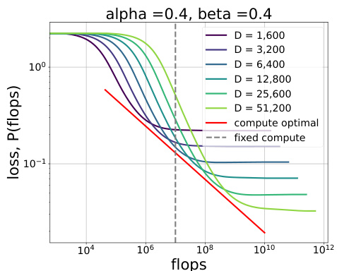
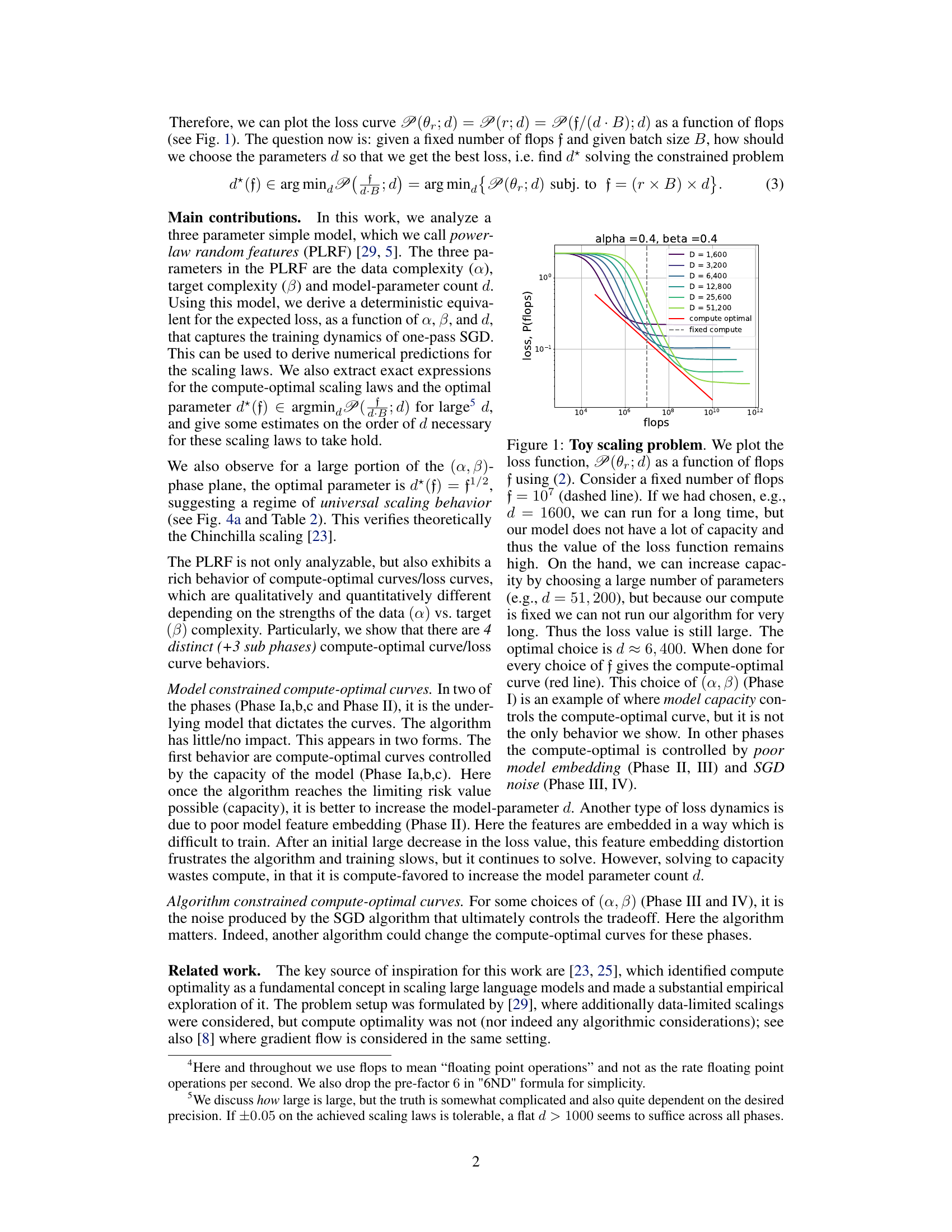
This figure illustrates a toy scaling problem. It shows how the loss function changes as a function of compute (flops) for different model sizes (d) with a fixed compute budget. The optimal model size that minimizes loss for a given compute budget is highlighted, demonstrating that there is an optimal model size to minimize loss given a fixed compute budget.

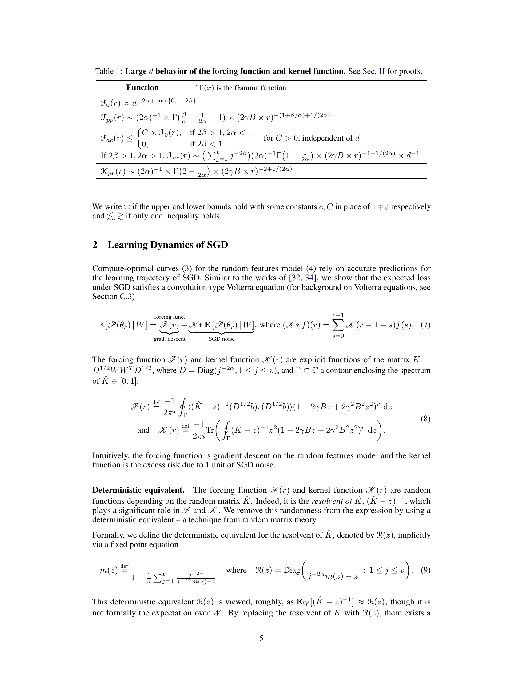
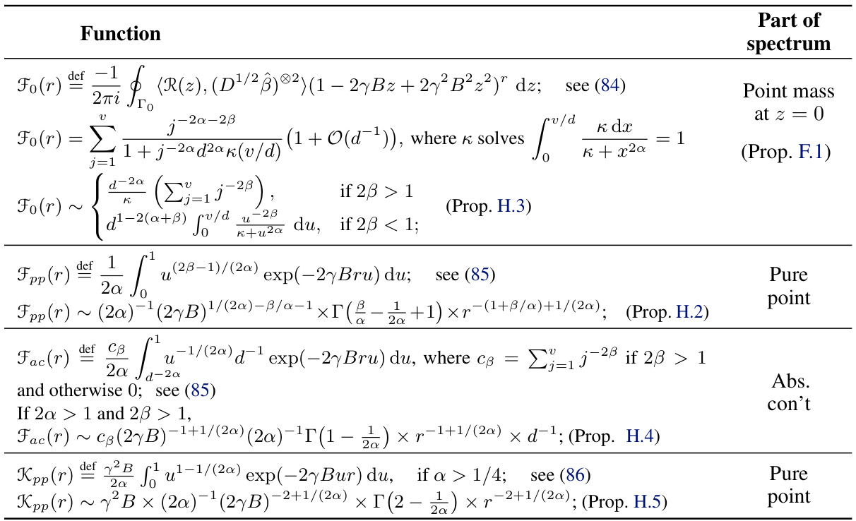
This table shows the asymptotic behavior of different components of the forcing function and the kernel function as the model parameter count (d) becomes large. These functions are crucial for understanding the learning dynamics of SGD, specifically for predicting the compute-optimal curves of the loss function. The table lists the asymptotic expressions for Fo(r), Fpp(r), Fac(r), and Kpp(r), which represent different aspects of the loss landscape, such as gradient descent, model capacity, and SGD noise. The asymptotic behavior is determined based on whether 2β > 1 or 2β < 1 and in the case that 2β > 1, there are different expressions for Fac(r) depending on whether 2α > 1 or 2α < 1. These results provide important theoretical building blocks for the analysis of the compute-optimal curves.
In-depth insights#
Compute-Optimal Laws#
The concept of “Compute-Optimal Laws” in the context of neural scaling explores how to optimally allocate computational resources for training neural networks. The core idea revolves around finding the model size that minimizes loss for a fixed computational budget, assuming effectively infinite data. This contrasts with traditional approaches that prioritize data limitations. Research in this area often involves analyzing how loss curves change with model size and compute, identifying phases of training behavior. Understanding these phases helps in determining optimal scaling laws (relationships between model parameters, compute, and loss). For instance, there might be regions where increasing model size drastically reduces loss, or where increasing compute beyond a certain point yields diminishing returns. The aim is to provide a theoretical framework for guiding resource allocation in training, thereby maximizing efficiency and minimizing training costs for large language models and other computationally intensive neural architectures. These laws are crucial for practical application, enabling efficient scaling of models within budget constraints. Further research would involve refining these laws to include more architectural details and optimizer considerations for more accurate and practical guidance in the field.
SGD Dynamics#
The section on “SGD Dynamics” would delve into the theoretical analysis of the stochastic gradient descent (SGD) algorithm’s behavior when applied to the power-law random features model. It would likely involve deriving a deterministic equivalent for the expected loss, potentially using techniques from random matrix theory to manage the randomness introduced by the stochasticity of SGD. This would likely involve establishing a relationship between the expected loss, the model parameters, the data complexity, and the target complexity. A key component would be the derivation of a Volterra equation, which would describe the trajectory of SGD’s iterates. Analyzing the Volterra equation would be crucial to understanding the dynamics of the learning process and how the algorithm navigates the loss landscape. The analysis might reveal insights into different phases of the optimization process, characterized by varying contributions of factors like optimizer noise, model capacity, and feature embedding. Ultimately, this section would provide the mathematical foundation for understanding the compute-optimal scaling laws and their dependence on algorithmic properties of SGD, rather than solely data or model capacity.
Four Phases#
The paper identifies four distinct phases in the neural scaling laws, characterized by how compute-optimal curves behave. These phases aren’t solely determined by model size, but also by the interplay between data complexity, target complexity, model capacity, optimizer noise, and feature embedding. Phase I highlights models limited by capacity, where increasing parameters directly improves performance. Phase II introduces the impact of feature embedding difficulties, where initial progress slows. Phase III shows optimizer noise as a significant factor and introduces universal scaling behavior. Finally, Phase IV is marked by the combined effects of capacity limitations and noise. Understanding these phases provides critical insights for optimizing training resource allocation and selecting model parameters to minimize loss given a fixed budget. The model used in the paper allows for the exact characterization of compute-optimal scaling laws across various phases, providing both theoretical and empirical evidence to support the findings. The existence of universal scaling in Phase III represents a particularly interesting and practically relevant insight.
Finite-Size Effects#
The section ‘Finite-Size Effects’ in this research paper would delve into the discrepancies between the theoretical model’s predictions and the results obtained from experiments with finite-sized neural networks. It would likely highlight the limitations of asymptotic analyses, which often assume infinitely large networks, and emphasize how these assumptions break down in practice. The discussion would likely cover the impact of finite data and computational resources on the observed scaling laws, potentially showing deviations from the theoretical power-law relationships for smaller models. The authors might explore the role of algorithmic noise (SGD) and its influence on performance, which becomes more pronounced in smaller networks. Furthermore, the effects of model architecture, such as the choice of activation functions or network depth, might be explored in the context of these limitations. A key insight could be the identification of thresholds or transition points marking the size beyond which asymptotic theory provides a reasonable approximation.
Future Research#
Future research directions stemming from this paper on compute-optimal neural scaling laws could fruitfully explore several avenues. Extending the theoretical framework to encompass more complex model architectures beyond the power-law random features model is crucial. This includes investigating the impact of depth, different activation functions, and other architectural choices on the scaling laws and optimal compute allocation. A deeper dive into the algorithmic aspects is also warranted, going beyond one-pass SGD to explore the effects of different optimizers, adaptive learning rates, and momentum on the compute-optimal curves. Investigating the impact of label noise and data distribution beyond power-law assumptions would enhance the model’s realism and applicability. Finally, empirical validation with diverse real-world datasets across various domains is essential to test the generalizability of the findings and uncover potential limitations or deviations from the theoretical predictions. This could include exploring low-resource scenarios where data is limited.
More visual insights#
More on figures
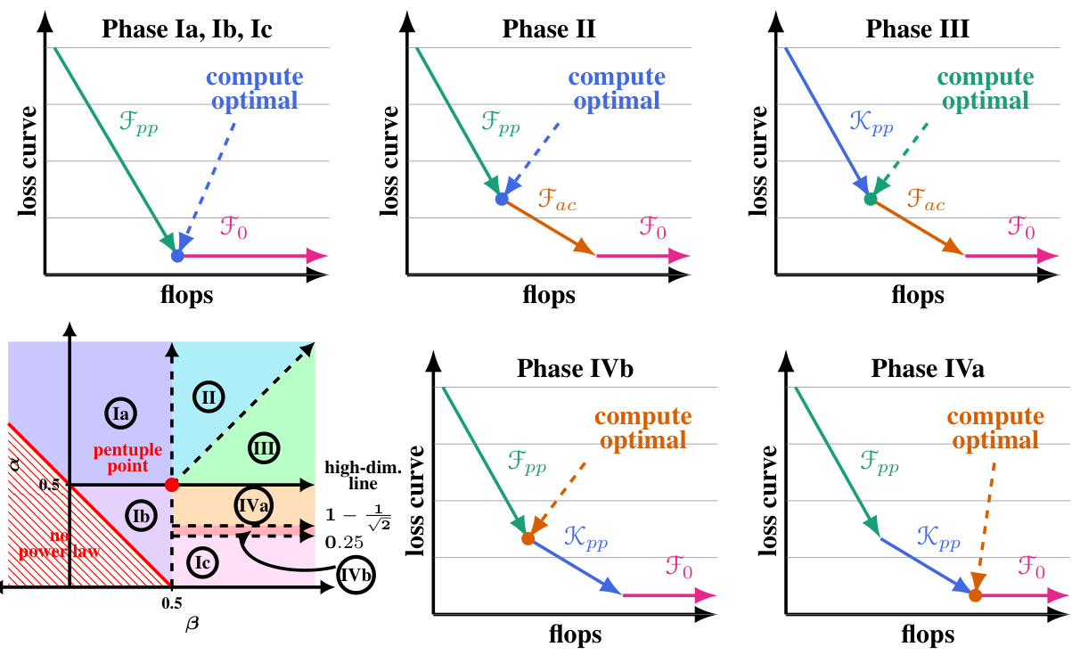
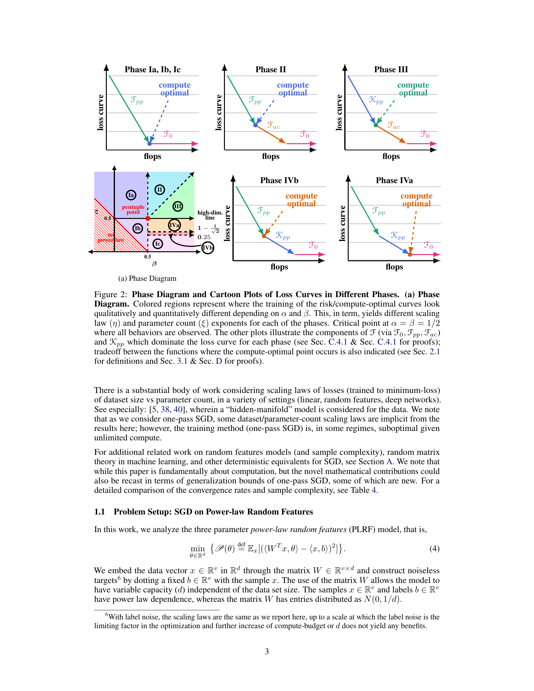
This figure shows a phase diagram and cartoon plots of loss curves for different phases in a three-parameter neural scaling model. The phase diagram illustrates regions where the training dynamics and optimal scaling laws change depending on data and target complexity. The cartoon plots visually represent how the loss curves behave for each phase, highlighting the dominant factors influencing the optimal parameter count and loss (model capacity, SGD noise, feature embedding).

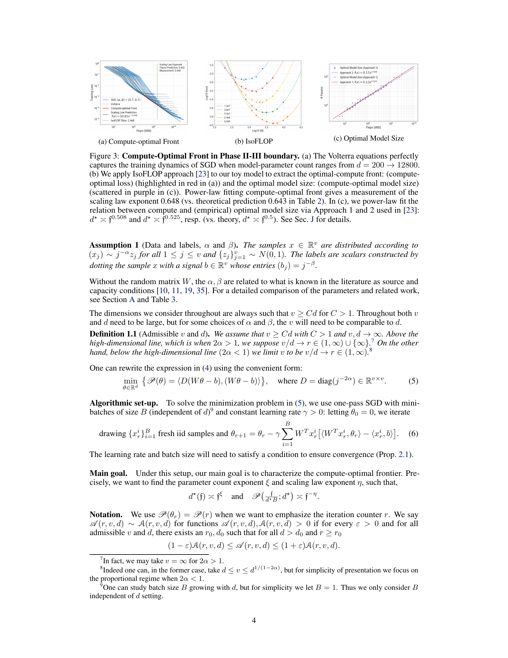
This figure demonstrates the compute-optimal front and model size in Phase II-III boundary of the parameter space. It compares empirical measurements with the theoretical predictions, validating the model’s accuracy. The figure includes plots showing the compute-optimal loss curve, iso-FLOP slices, and the relation between optimal model size and compute.
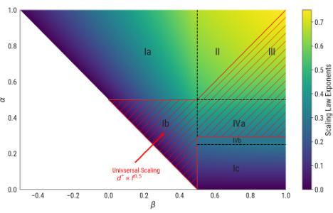
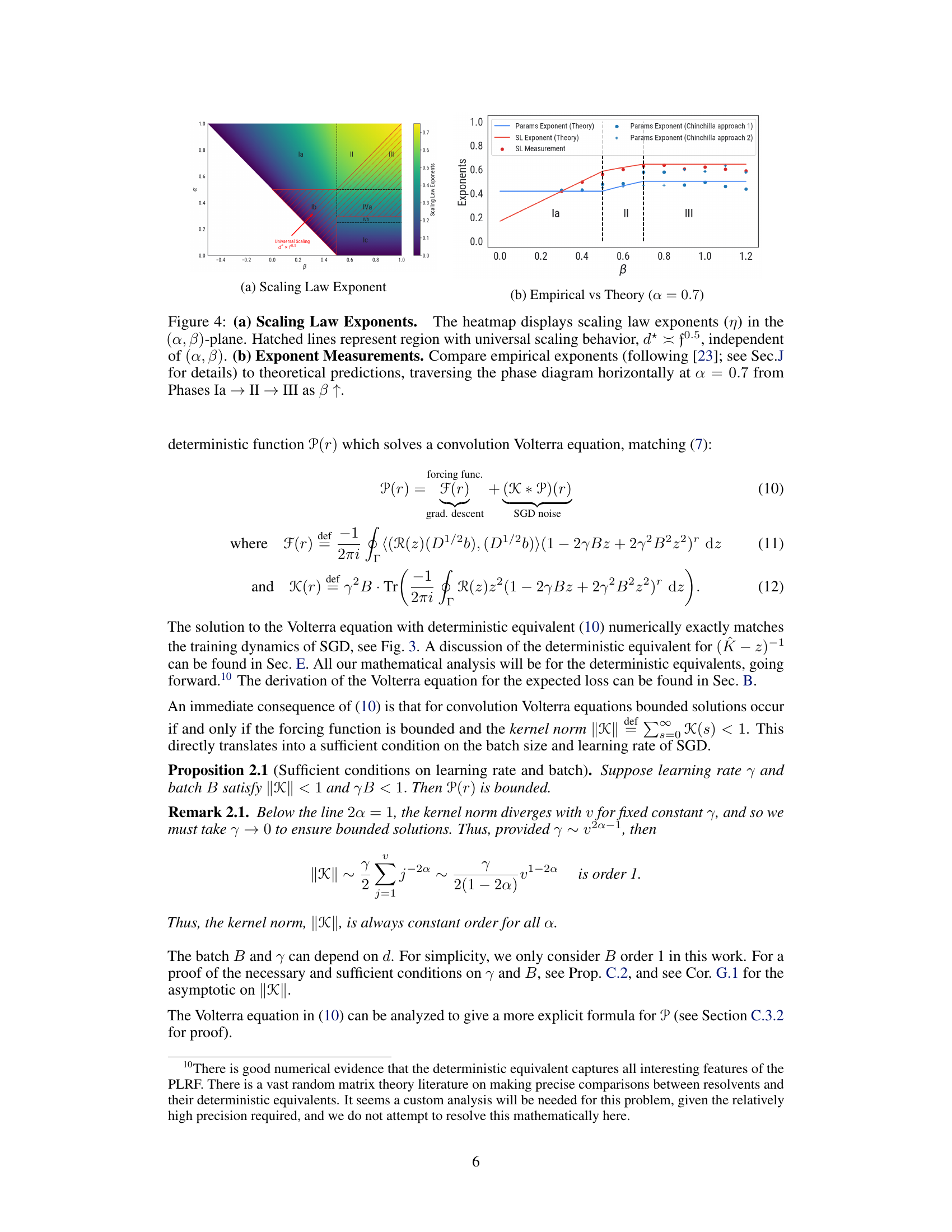
This figure shows the scaling law exponents (η) and parameter count exponents (ξ) in the (α,β)-plane. The heatmap (a) shows the scaling law exponent η and the parameter count exponent ξ for each phase. The hatched lines show the region where the universal scaling behavior d* = f0.5 is observed, independent of the values of α and β. The plot (b) compares the empirical exponents (measured using the method in [23]) and theoretical predictions. The plot shows that the theoretical predictions are consistent with the empirical measurements, especially when the data complexity α is high and the target complexity β is low.
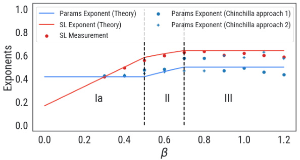
This figure shows the scaling law exponents in the (α, β)-plane. The heatmap in (a) visualizes how the scaling law exponent changes depending on the data complexity (α) and target complexity (β). The hatched lines indicate a region where the scaling behavior is universal, meaning d* (optimal parameter count) is always proportional to f0.5 (flops) regardless of α and β values. Part (b) compares these theoretical predictions with empirical measurements obtained by traversing the phase diagram horizontally (α = 0.7) while increasing β. The graph demonstrates how the measured exponents transition through different phases (Ia, II, III) as β increases.

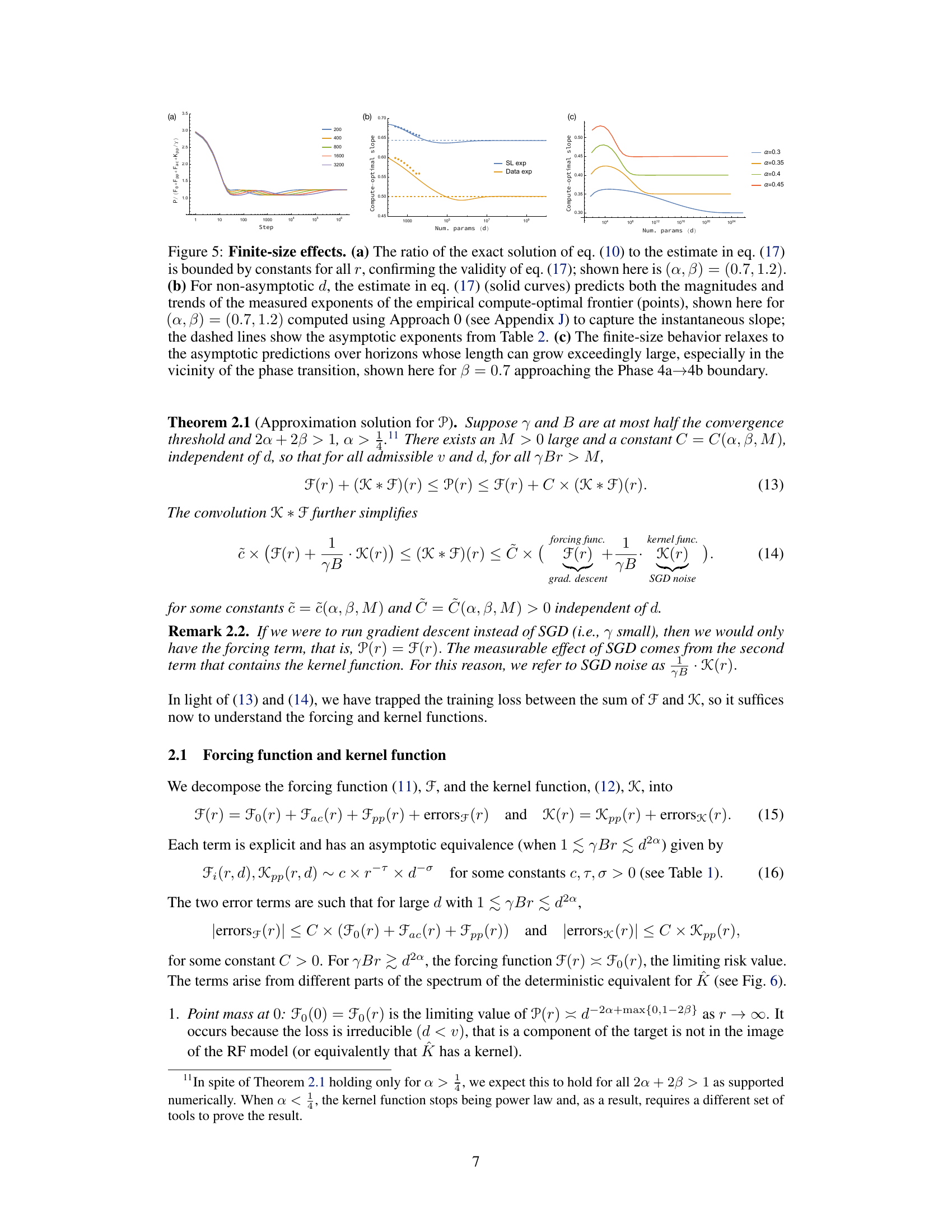
This figure demonstrates the finite-size effects on the compute-optimal curves. Panel (a) shows the ratio of the exact solution of the Volterra equation to an estimate, confirming the estimate’s validity. Panel (b) compares the estimate with empirical measurements, showing good agreement even for non-asymptotic d values. Panel (c) demonstrates that the finite-size effects diminish over longer training times, particularly near phase transitions.
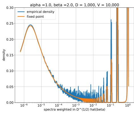
This figure compares the empirical and theoretical spectra of the random matrix K = D^(1/2)WWT D^(1/2), weighted by D^(1/2)hat(β). The empirical spectra are obtained by averaging over 100 randomly generated matrices W, while the theoretical spectra are computed using the resolvent formula (9) and a Newton method. The figure shows the three distinct parts of the spectrum: a point mass at z=0, pure point outliers, and an absolutely continuous part. The point mass at z=0 was manually removed from the empirical spectra before the comparison.
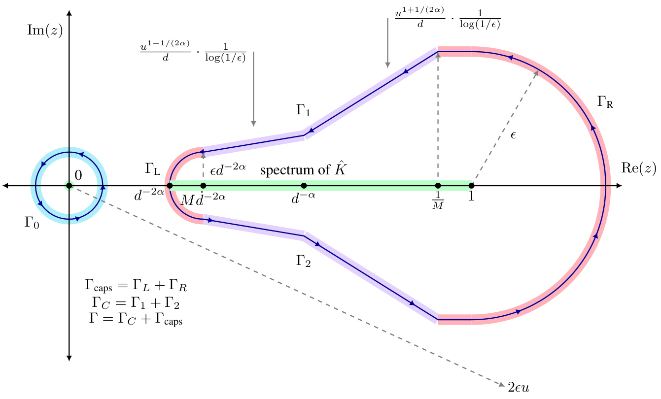
This figure shows the contour used to estimate the forcing and kernel functions. The contour is split into three parts: Γο, Γc, and Γcaps. Γο is a small contour around 0, Γc is the contour for the bulk of the spectrum of K, and Γcaps connects the ends of Γc. The spectral gap occurs at d−2α. The figure also shows how the contour changes behavior at d−α due to the transition from pure points to absolutely continuous spectrum.

This figure shows the scaling law exponents in the (α, β) plane. The heatmap shows the scaling law exponent values for different combinations of α and β. The hatched lines in the heatmap indicate the universal scaling regime where the optimal parameter count is proportional to the square root of the compute budget. The second part of the figure shows a comparison of empirical and theoretical exponent measurements across different phases for a fixed α of 0.7. As β increases, the system transitions through phases Ia, II, and III. The plot compares the empirical scaling law exponents measured using a method from a previous study to the theoretical predictions derived in the current paper.
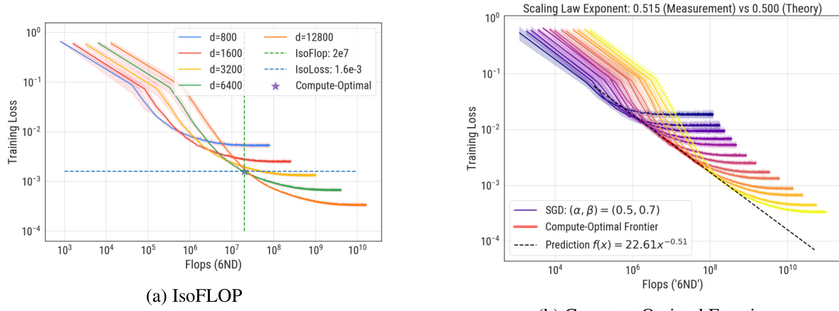
Figure 3 shows the compute-optimal front in the boundary between Phase II and III. Panel (a) shows that the Volterra equation captures the training dynamics of SGD across a range of model sizes. Panel (b) uses the IsoFLOP method to extract the compute-optimal front, shown in red and panel (c) shows the power-law fit to the optimal model size. The scaling law exponent was measured as 0.648, similar to the theoretical prediction of 0.643.
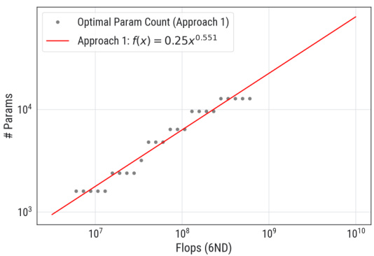
This figure shows the results of applying the IsoFLOP approach to the toy model used in the paper. Panel (a) displays the compute-optimal front, which is a curve showing the optimal loss achievable for a given compute budget. This curve is compared to the theoretical predictions from the Volterra equations. Panel (b) focuses on a specific IsoFLOP slice (a vertical line in (a)) to show the relationship between model size and loss. Panel (c) fits a power law to the optimal model size across various compute budgets, comparing it to existing theoretical predictions. The figure validates the theoretical predictions with experimental results, especially for the scaling law exponent.
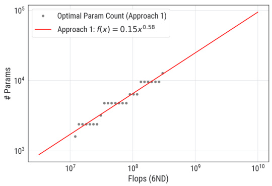
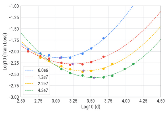
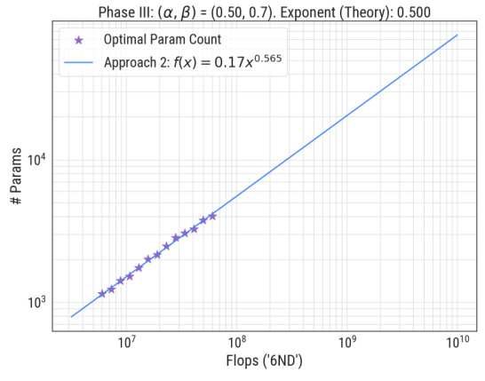
This figure shows how sensitive the parameter count exponent is to the choice of IsoFLOP window used in Approach 1. The plots show the optimal parameter counts (number of parameters) plotted against the compute budget (in FLOPs) for two different IsoFLOP windows: [1e6, 1e8] (a) and [2e6, 0.5e8] (b). For both plots, the data points represent empirical measurements obtained from training runs. The lines represent power law fits to the data, where the exponent of the power law represents the parameter count exponent. The different exponents in (a) and (b) highlight that the exponent changes when different windows are selected. This implies that the value of the parameter count exponent is sensitive to this hyperparameter.
This figure shows the results of applying the IsoFLOP approach to a toy model to extract the compute-optimal front and optimal model size. Panel (a) shows the compute-optimal front, which is the curve connecting the minimum losses achievable for different compute budgets. Panel (b) shows how the scaling law exponent is measured from the compute-optimal front via power-law fitting. Panel (c) displays a power-law fit of optimal model size as a function of compute budget. The results are compared to theoretical predictions, showing good agreement between measurement and theory.
This figure shows the results of applying the IsoFLOP method to a toy model. Panel (a) demonstrates how well the Volterra equations capture the training dynamics of SGD. Panel (b) shows the compute-optimal front and the associated optimal model size. A power-law fit of the compute-optimal front yields a scaling law exponent, which is compared to a theoretical prediction. Panel (c) shows a power-law fit of the relationship between compute and optimal model size, comparing the empirical results to theoretical predictions.
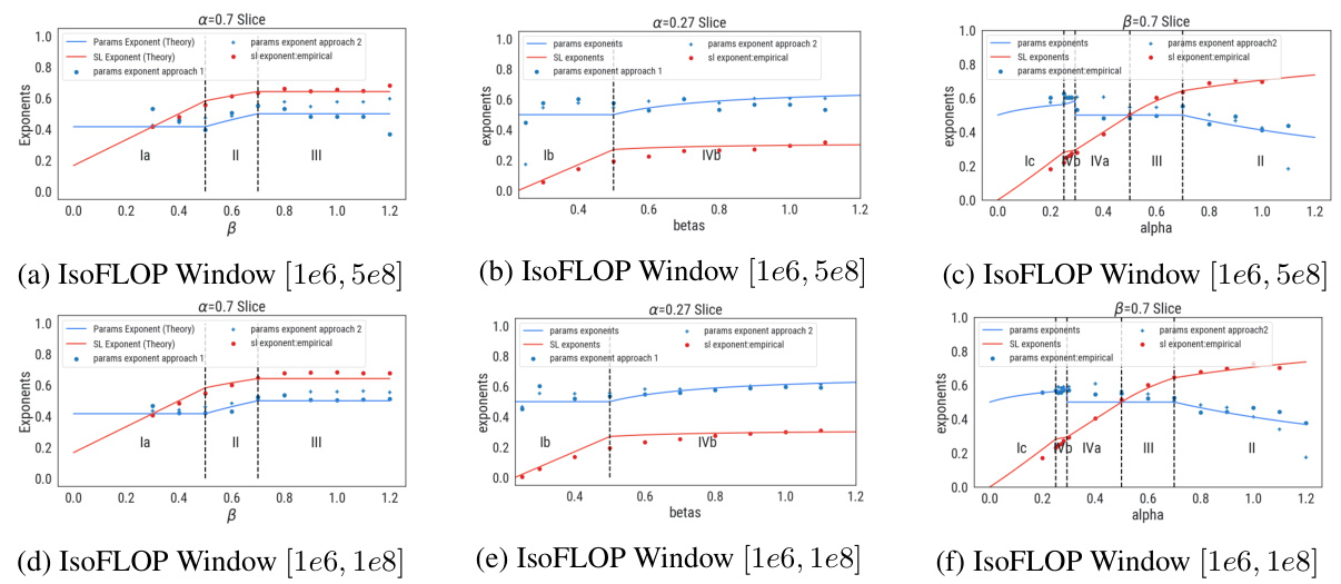
This figure shows the scaling law exponents in the (α, β)-plane, which are obtained from the theoretical analysis using the Volterra equation. The heatmap in (a) shows that the scaling law exponents depend on the data complexity α and target complexity β. The hatched lines represent the region with universal scaling behavior, d* = f0.5, which is independent of α and β. The plot (b) compares the empirical exponents with the theoretical predictions. The empirical exponents are obtained from the experiments using the Chinchilla approach, and the theoretical predictions are obtained from the theoretical analysis.

This figure shows the compute-optimal front obtained from the Volterra equations and the IsoFLOP approach. Panel (a) shows the training loss as a function of floating-point operations, highlighting the compute-optimal loss. Panel (b) shows the IsoFLOP curve fitting to obtain the scaling law exponent. Panel (c) shows the optimal model size, comparing the empirical results from the IsoFLOP approach with theoretical predictions.
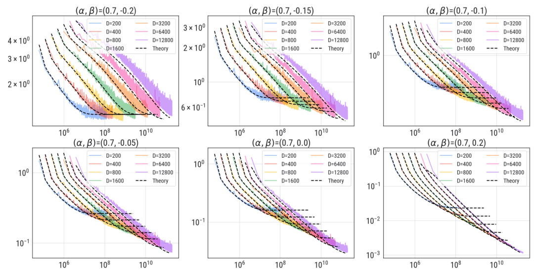
This figure shows the experimental results for negative values of β. It presents multiple plots, each corresponding to a different β value ranging from -0.2 to 0.2, with α held constant at 0.7. For each β, multiple curves represent different model parameter counts (d), compared to the theoretical prediction from the Volterra equation. The plots visually demonstrate the close agreement between the theoretical predictions and empirical observations across various values of β, validating the theoretical model’s ability to accurately capture the learning dynamics.
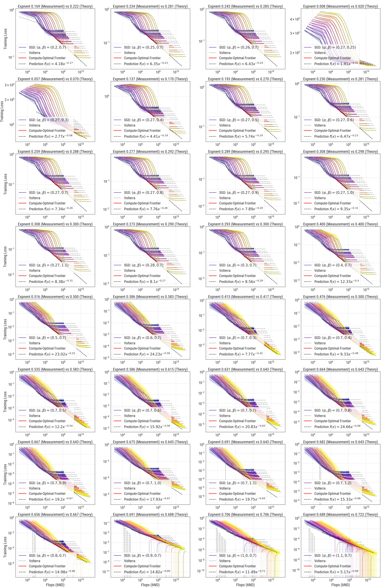
This figure shows the compute-optimal front and optimal model size obtained from the three-parameter neural scaling model. The left panel (a) shows the compute-optimal front, which is the curve representing the lowest loss for each compute budget. The middle panel (b) shows how the model size (number of parameters) changes to achieve this optimal loss in the Phase II-III boundary. The right panel (c) presents a power-law fit for the optimal model size as a function of the compute budget, comparing the empirical findings with the theoretical prediction, validating the scaling law exponent of approximately 0.5.
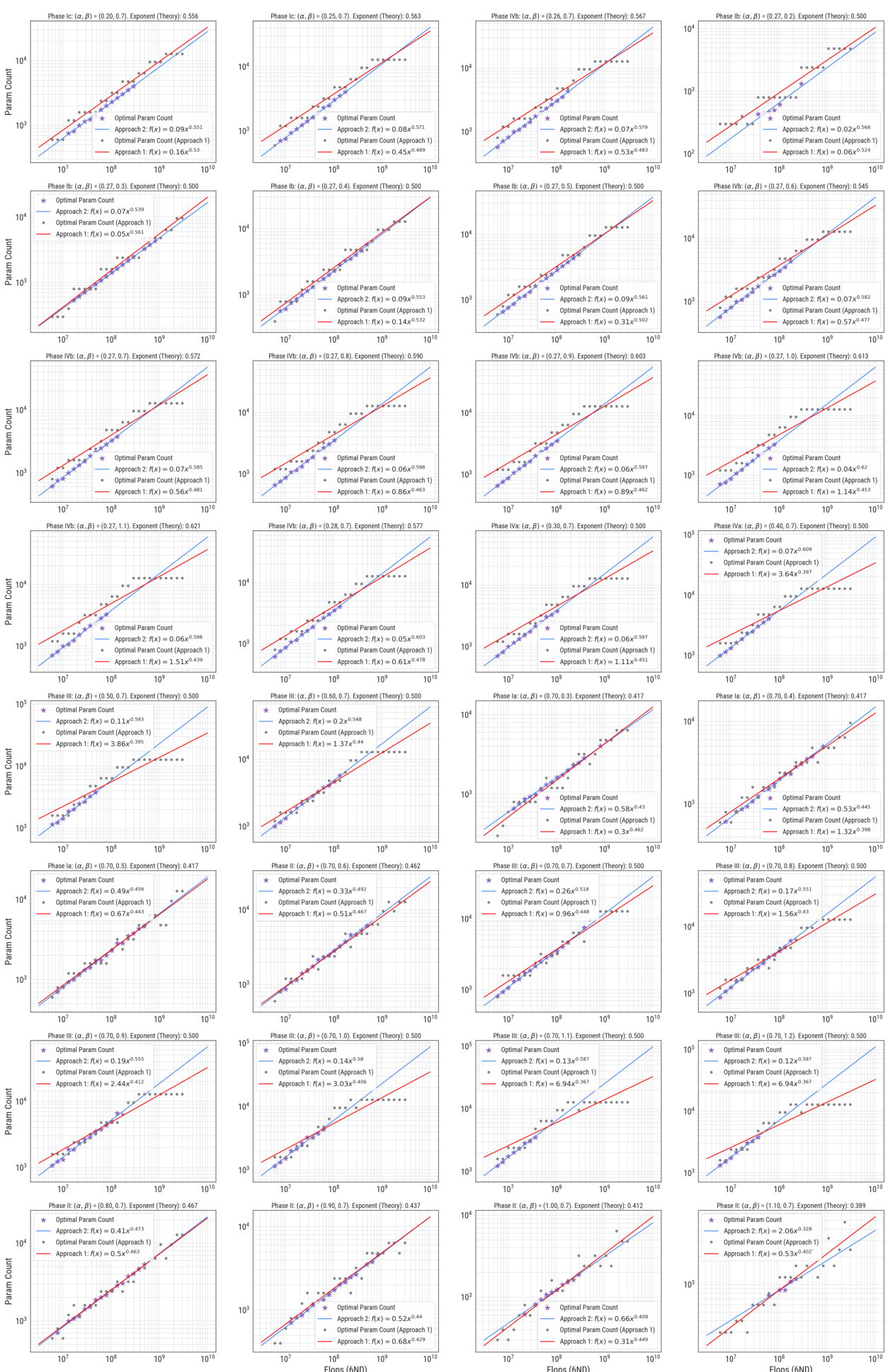
This figure shows the results of applying the IsoFLOP approach to the toy model, comparing theoretical predictions with empirical measurements. Panel (a) shows the compute-optimal front using the Volterra equations. Panels (b) and (c) showcase power-law fitting of compute-optimal loss and model size respectively, validating the theoretical predictions.
More on tables
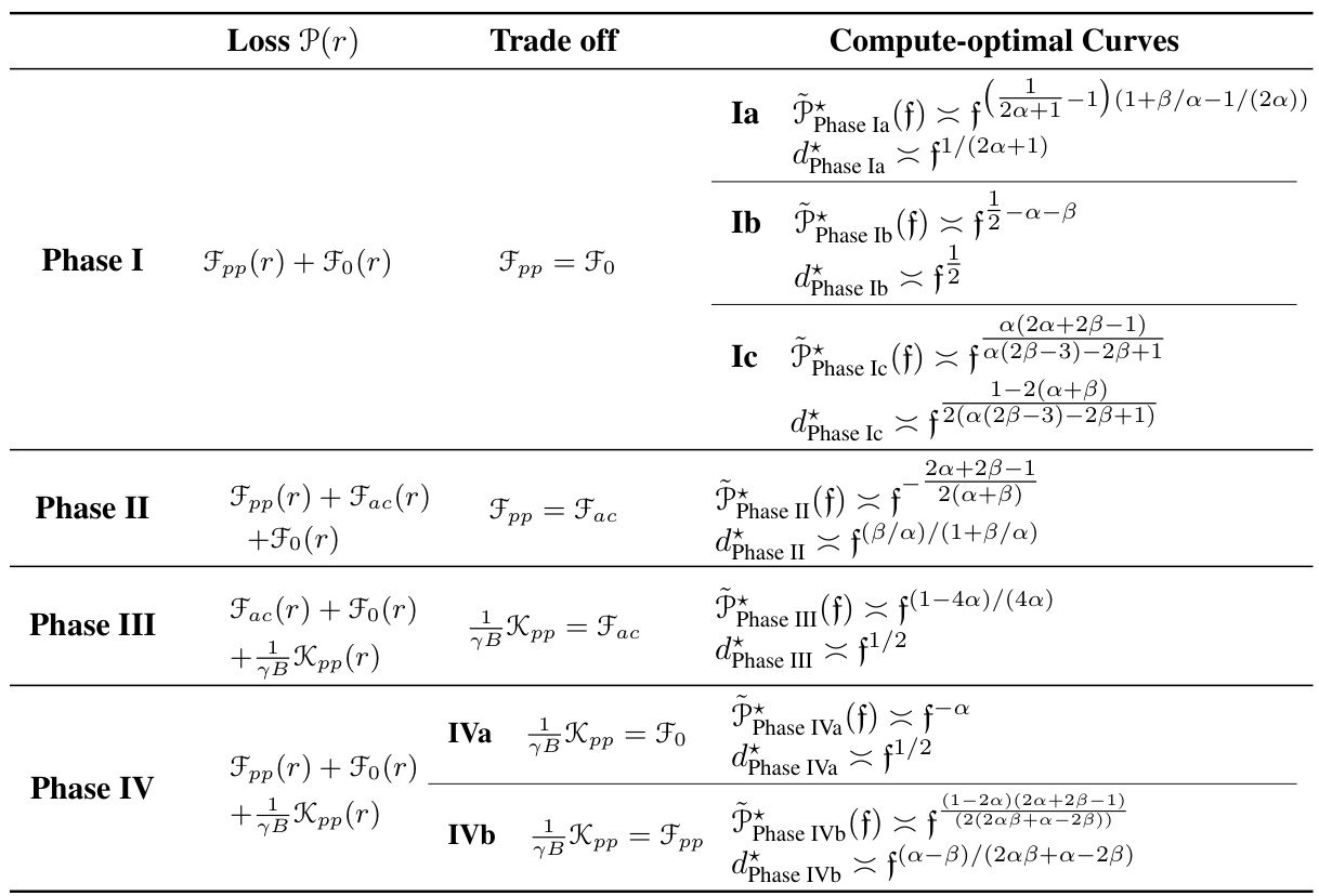
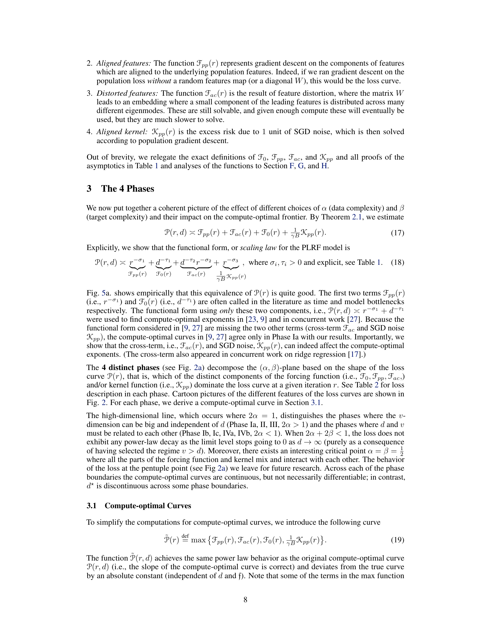
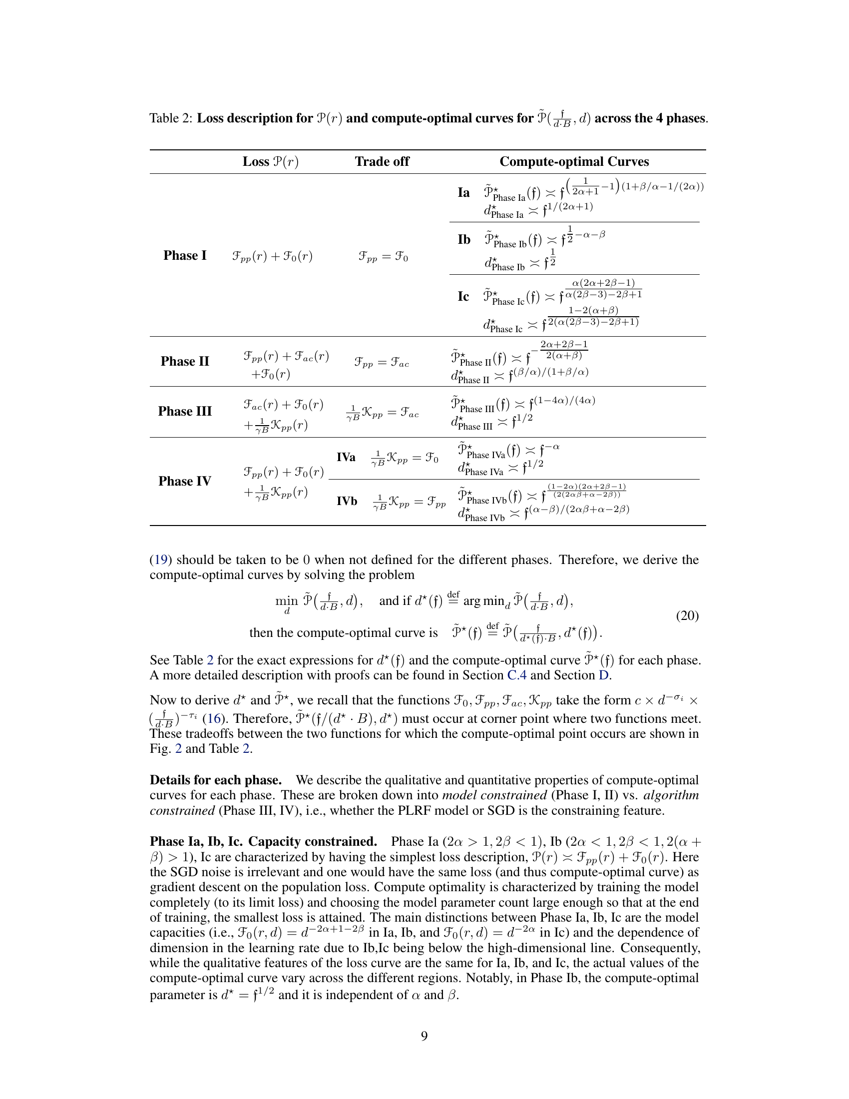
This table summarizes the four phases of compute-optimal curves identified in the paper. For each phase, it provides a description of the loss function P(r), the trade-off between the dominant terms in the loss, and the resulting compute-optimal curves (P*(f) and d*(f)) derived using a specific three parameter model.

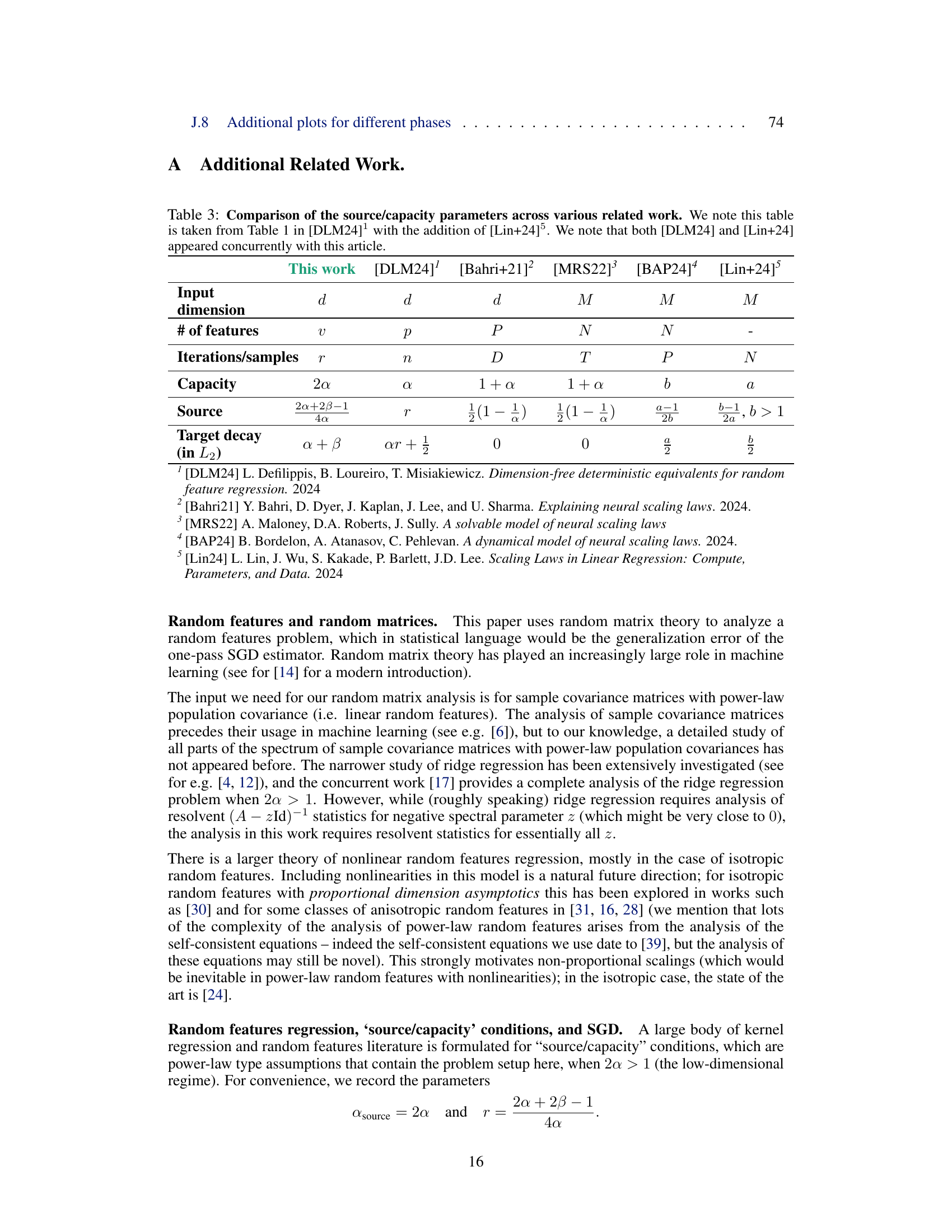
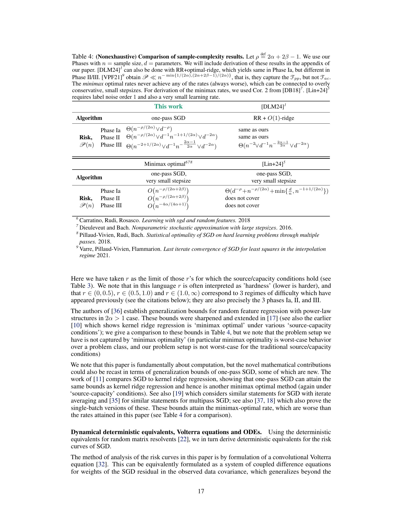
This table compares the notation and parameters of different works related to the paper. It shows how the input dimension, number of features, iterations/samples, capacity, source, and target decay parameters are defined and denoted in various papers, including the current work and several others. The table aims to clarify the relationships between these parameters across different research efforts in neural scaling laws.
This table summarizes the key characteristics of the four phases identified in the paper regarding compute-optimal neural scaling laws. For each phase, it provides a description of the loss function P(r) in terms of the dominant components (Fpp, Fac, Fo, Kpp), highlighting the trade-off between these components that determines the compute-optimal behavior. Furthermore, it presents the compute-optimal curves for P(, d), including the expressions for the optimal parameter count d*(f) and the compute-optimal loss P*(f).
This table summarizes the characteristics of the four phases identified in the paper, namely Phase I, II, III, and IV. For each phase, it provides a description of the loss function P(r), indicating which terms (Fpp(r), Fac(r), Fo(r), and Kpp(r)) are dominant. Additionally, it specifies the trade-off between these terms that leads to compute-optimal curves, and it gives the resulting expressions for the compute-optimal curves, P*(f), and the optimal parameter count, d*(f). The table helps to understand how the different components of the loss function interact and how they shape the compute-optimal behavior in each phase.
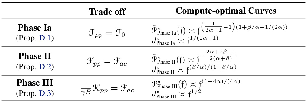
This table summarizes the characteristics of the four phases identified in the paper regarding compute-optimal neural scaling laws. For each phase, it provides a description of the loss function ((\mathcal{P}(r))), the trade-off between the dominant terms in the loss function, the compute-optimal curves ((\tilde{\mathcal{P}}(f, d))), and the compute-optimal parameter count ((d^*(f))). The phases are categorized by the relative importance of model capacity, optimizer noise, and embedding of features, leading to distinct scaling behaviors. The table helps to understand the different regimes and predict the optimal neural network size based on available computational resources.
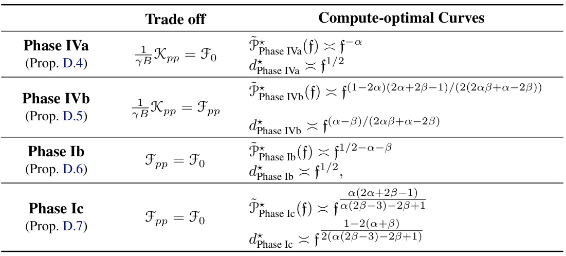
This table summarizes the key characteristics of the four phases identified in the paper’s compute-optimal analysis. For each phase, it provides a description of the loss function ((\mathcal{P}(r))), the trade-off that determines the compute-optimal point, and the resulting compute-optimal curves and parameter count exponents. The table helps to understand how different combinations of data complexity (α) and target complexity (β) lead to distinct behaviors in the compute-optimal scaling laws. Specific mathematical expressions for the optimal curves and exponents are given in the paper.
Full paper#
