↗ OpenReview ↗ NeurIPS Proc. ↗ Chat
TL;DR#
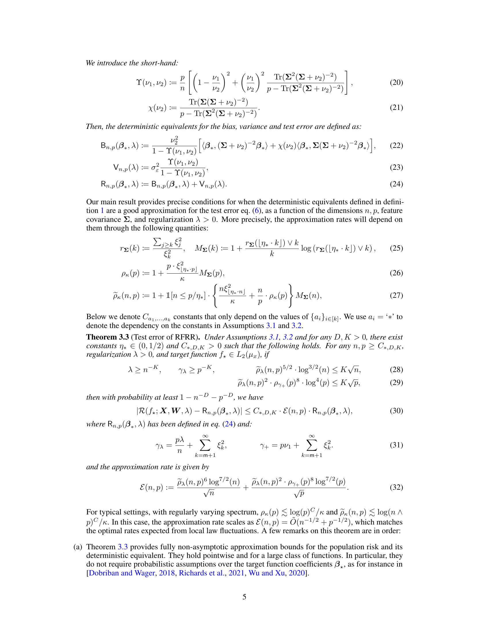
Overparametrized neural networks’ ability to generalize despite perfect training data interpolation has puzzled researchers. Understanding generalization in such models is crucial. Prior works often relied on asymptotic analysis, limiting their practical applicability. This work tackled these issues.
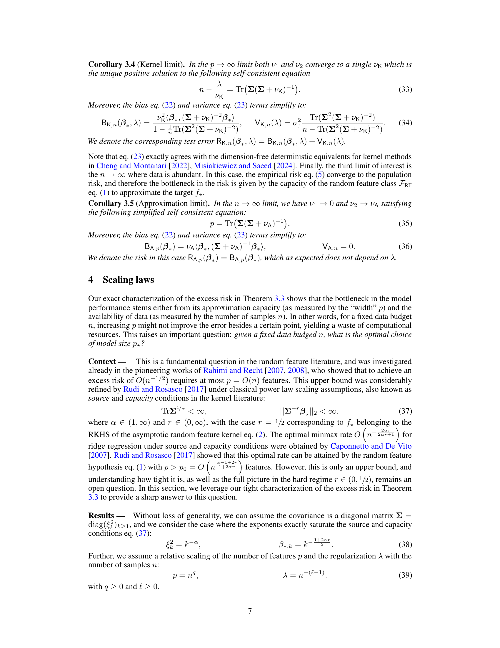
This paper introduces a novel, dimension-free deterministic equivalent for random feature regression’s test error. This means they developed a closed-form approximation highly accurate even with high-dimensional or infinite-dimensional features. This method is validated using real and synthetic data, offering new insights into the relationship between overparametrization, feature map properties, and generalization performance. They also derived sharp error rates, demonstrating the model’s efficiency and advancing our understanding of neural network generalization.
Key Takeaways#
Why does it matter?#
This paper is crucial for researchers working on random feature regression and neural network generalization. It provides dimension-free deterministic equivalents, enabling precise non-asymptotic analysis of generalization error. The findings offer significant insights into optimal minimax rates and scaling laws, addressing fundamental questions about overparametrized models and paving the way for improved learning algorithms.
Visual Insights#
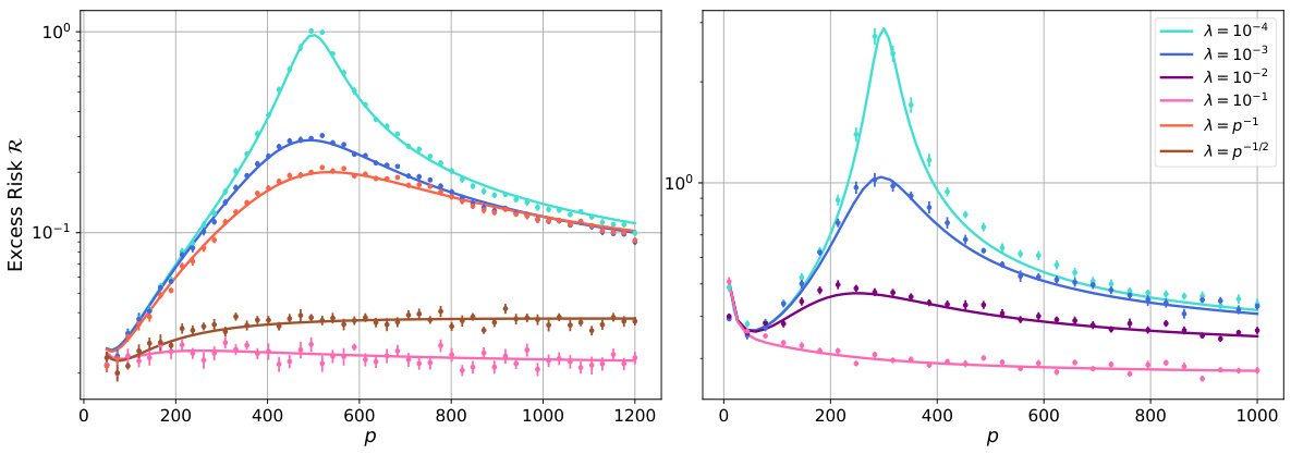
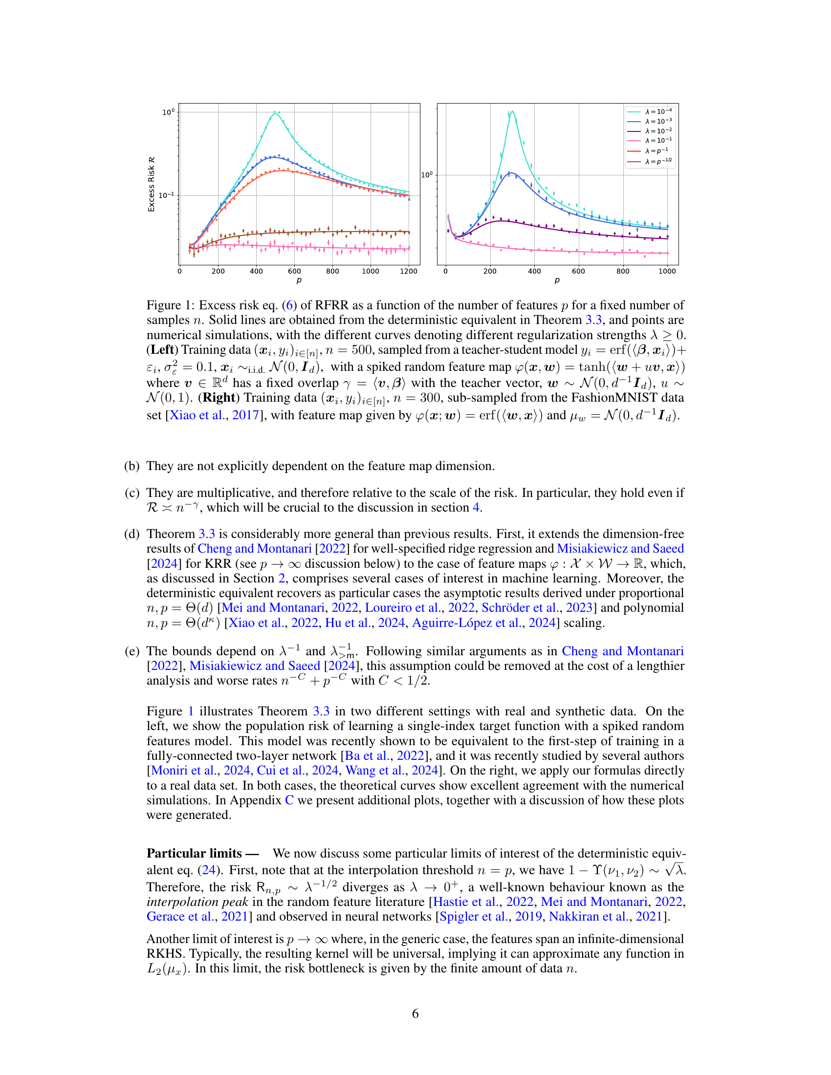
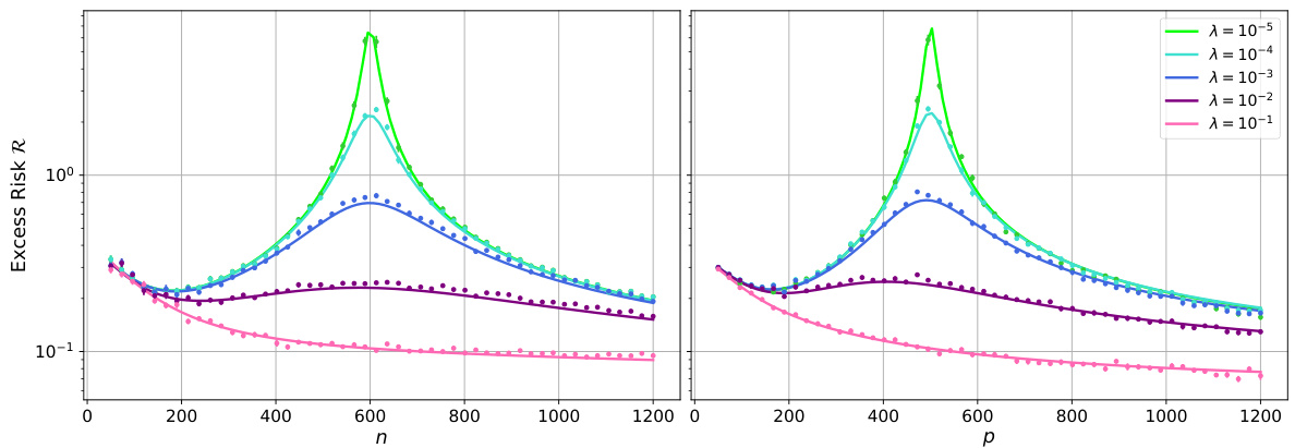
The figure shows the excess risk of random feature ridge regression (RFRR) as a function of the number of features (p) for a fixed number of samples (n). The solid lines represent the theoretical predictions from a deterministic equivalent derived in the paper (Theorem 3.3), while the points are the results of numerical simulations. Different lines represent different regularization strengths (λ). The left panel shows results using a teacher-student model with a spiked random feature map, while the right panel utilizes data from the FashionMNIST dataset and a different feature map.

This table compares the notations used for describing the scaling laws in different works, including the current work and three other prominent papers. It highlights the differences in notation for key parameters such as input dimension, number of features, number of samples, capacity, source, and target decay, facilitating a better understanding of the various scaling laws discussed in the paper.
In-depth insights#
Dimension-Free RFRR#
The concept of “Dimension-Free RFRR” suggests a significant advancement in random feature ridge regression (RFRR). Traditional RFRR analyses often rely on asymptotic approximations, making their validity dependent on the feature map dimension. A dimension-free approach, however, eliminates this dependency, providing more robust and broadly applicable results. This implies that the theoretical guarantees of the RFRR model are independent of the dimensionality of the feature space, which is a critical improvement. Non-asymptotic guarantees are particularly important, offering strong confidence in the model’s performance even for finite sample sizes, unlike many asymptotic approaches. The achievement of dimension-free results for RFRR would likely involve novel mathematical techniques that address the inherent complexities of high-dimensional data. Sharper excess risk rates would be another key benefit, enabling more accurate prediction of generalization error. Ultimately, a “Dimension-Free RFRR” framework would provide more reliable and practical tools for real-world applications. This is especially valuable in domains dealing with inherently high-dimensional or infinite-dimensional feature spaces.
Deterministic Equiv.#
The section on “Deterministic Equiv.” likely details a core methodological contribution of the research paper. It almost certainly presents a deterministic approximation of a typically stochastic quantity, such as the risk or generalization error in a random feature regression model. This approximation simplifies the analysis, providing a closed-form expression that bypasses the need for computationally expensive simulations or asymptotic analysis. The approximation’s accuracy likely depends on fulfilling certain concentration conditions (assumptions). The authors probably demonstrate the quality of their approximation both theoretically, using concentration inequalities to bound the error, and empirically by comparing the predictions to experimental results on various datasets. Crucially, dimension-free aspects are highlighted, meaning the accuracy of the approximation is not directly hampered by the dimensionality of the feature space. This is a significant result as it facilitates analysis in high-dimensional settings, relevant to many machine learning applications. Overall, this “Deterministic Equiv.” section is vital in establishing the practical applicability and theoretical tractability of the proposed model.
Scaling Laws#
The section on “Scaling Laws” in this research paper delves into the relationship between model performance and key resources such as data amount and model size. It investigates how the excess risk (error) scales with these factors under specific assumptions on the target function and feature spectrum. Power-law scaling assumptions, also known as source and capacity conditions, play a crucial role, defining how quickly the target function and feature map eigenvalues decay. The authors aim to derive a tight expression for the minimum number of features needed to achieve the optimal minimax error rate, thereby establishing the most efficient use of model capacity. The theoretical findings are supported by numerical simulations with real and synthetic data, illustrating the practical implications of these scaling laws. The paper demonstrates that the optimal performance depends on achieving a balanced trade-off between model complexity (number of features) and data availability, a dimension-free characterization that moves beyond previous asymptotic results.
Concentration Prop.#
The heading ‘Concentration Prop.’ likely refers to a concentration inequality or theorem used within a statistical learning or high-dimensional probability context. Such propositions are crucial for establishing generalization bounds. They essentially state that a complex random variable (e.g., an empirical risk) concentrates around its mean or expectation with high probability, often exponentially fast. This is essential because directly working with the random variable is often intractable. Concentration inequalities allow for replacing the random variable with a deterministic equivalent, simplifying analysis and obtaining tight bounds. The choice of specific concentration inequality depends on the specific properties of the random variable in question, and the proof of the main result hinges on the ability to demonstrate that the concentration property holds. The strength of the concentration result dictates the quality of the generalization bounds: tighter concentration leads to sharper generalization bounds. Furthermore, the ‘Concentration Prop.’ is likely central to proving that the dimension-free deterministic equivalent for the risk accurately approximates the test error of a model.
Future Directions#
The study of random feature regression (RFRR) is ripe for further investigation. Future research should focus on relaxing the restrictive assumptions, particularly the concentration inequalities on feature map eigenfunctions, to make the theoretical results more broadly applicable to real-world scenarios and non-linear feature maps. Empirical validation across diverse datasets with varying dimensions is crucial to assess the robustness and generalizability of the deterministic equivalent approximations. Furthermore, extending the analysis to other learning tasks and exploring the impact of different optimization algorithms is important. A deeper investigation into the interplay between the spectral properties of the feature maps, the target function decay, and the optimal number of features is needed. This includes determining the minimum number of features that achieve optimal minimax error rates in diverse settings, particularly for functions that do not reside in the RKHS of the limiting kernel. Finally, incorporating the computational aspects, such as the scaling laws observed in large-scale neural networks, into the theoretical framework could provide a more comprehensive understanding of RFRR’s generalization performance.
More visual insights#
More on figures
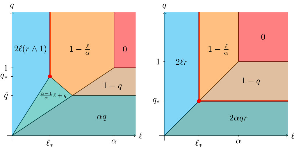
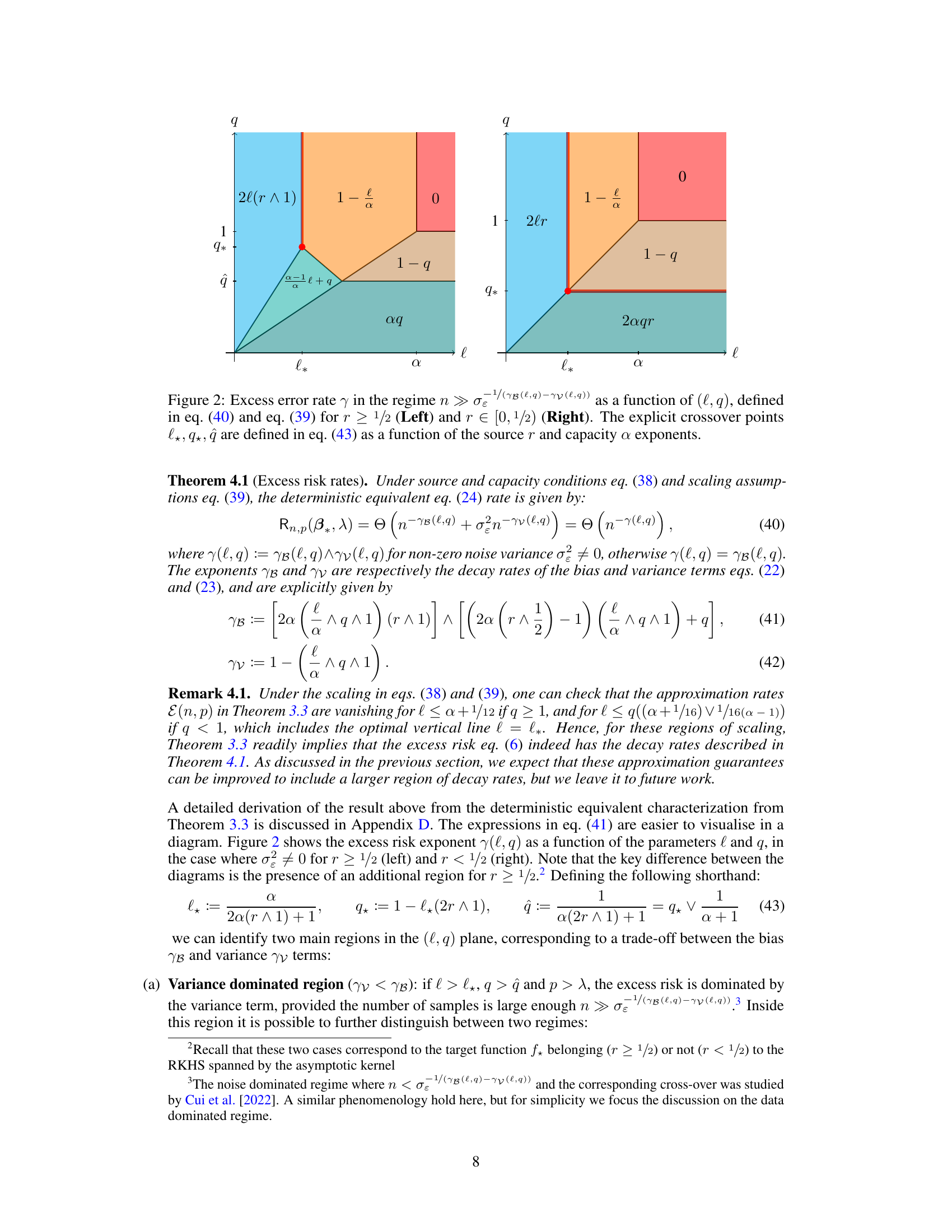
This figure shows the excess error rate as a function of the scaling parameters l and q for different values of the source exponent (r) and capacity exponent (a). The left panel shows the case where r >= 1/2, while the right panel shows the case where r is between 0 and 1/2. Different colors represent different regions with different dominant factors in the excess risk (bias vs variance). The figure illustrates the trade-offs between the bias and variance terms under different scaling regimes and helps to identify the optimal scaling parameters for achieving optimal excess risk rate.
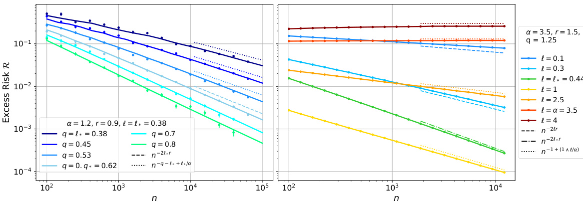
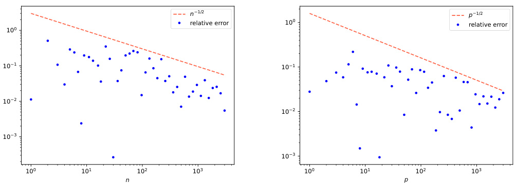
This figure displays the excess risk of random feature ridge regression as a function of the number of samples (n) under specific source and capacity conditions. It compares the theoretical predictions from the deterministic equivalent (solid lines) with numerical simulations (points) for different regularization strengths and numbers of features. The dashed and dotted lines represent analytical rates from a different theorem, and the colors correspond to different regions defined in a previous figure (Fig 2). The figure highlights the different scaling regimes of the excess risk and the crossover points between them. The left panel shows a smaller α and r<1/2 while the right panel show a larger α and r≥1/2.
The figure shows the excess risk of random feature ridge regression (RFRR) as a function of the number of features (p) for a fixed number of samples (n). The solid lines represent the theoretical predictions from a deterministic equivalent derived in the paper, while the points are from numerical simulations. Different lines represent different regularization strengths (λ). The left panel uses synthetic data generated by a teacher-student model with a spiked random feature map, while the right panel uses real data from the FashionMNIST dataset. The figure empirically validates the accuracy of the theoretical approximation.
The figure shows the excess risk of random feature ridge regression (RFRR) as a function of the number of features (p) for a fixed number of samples (n). It compares theoretical predictions (solid lines) derived from a deterministic equivalent (Theorem 3.3) with numerical simulations (points). Different curves represent different regularization strengths (λ). The left panel displays results for a teacher-student model with a spiked random feature map, while the right panel uses data from the FashionMNIST dataset with a different feature map.
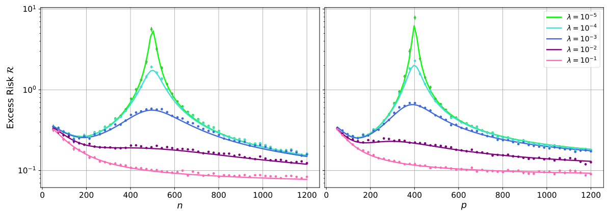
This figure displays the excess risk of random feature ridge regression (RFRR) as a function of the number of features (p) for a fixed number of samples (n). The solid lines represent the theoretical predictions from the deterministic equivalent derived in the paper (Theorem 3.3), while the points show the results of numerical simulations. Different colors represent different regularization strengths (λ). The left panel uses synthetic data generated from a teacher-student model with a spiked random feature map, while the right panel uses real data from the FashionMNIST dataset.
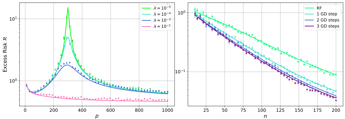
This figure compares the excess risk of random feature ridge regression obtained from simulations and the deterministic equivalent derived in the paper. The left panel shows the results for MNIST data with different regularization strengths, while the right panel demonstrates the impact of gradient descent iterations on the model’s performance using a teacher-student model.
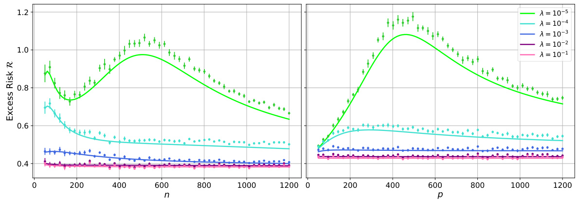
The figure shows the excess risk of random feature ridge regression (RFRR) as a function of the number of features (p) for a fixed number of samples (n). It compares theoretical predictions (solid lines) derived from a deterministic equivalent (Theorem 3.3) to numerical simulations (points). Different curves represent different regularization strengths (λ). The left panel uses synthetic data from a teacher-student model, while the right panel uses real data from the Fashion-MNIST dataset.
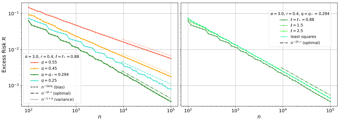
This figure shows the excess risk of random feature ridge regression as a function of the number of samples (n) under specific source and capacity conditions. The plots illustrate the theoretical predictions (solid lines) from Theorem 3.3 and numerical simulations (points). Different lines represent different regularization strengths (λ) and numbers of features (p), which are scaled relative to n. The plots also show the theoretical decay rates of the bias and variance terms, and highlight the different scaling regimes (variance-dominated, bias-dominated) and the optimal decay rate. The left subplot displays the crossover between different regimes while the right one shows the optimal decay rate.
Full paper#
