Statistical Multicriteria Benchmarking via the GSD-Front

jXxvSkb9HD

Christoph Jansen et el.

TL;DR
#

Comparing classifiers is challenging due to the vast number of existing methods and the need to consider multiple quality metrics simultaneously. Existing approaches, like using a single weighted metric or focusing solely on the Pareto-front, often lack reliability because they either ignore the distribution of datasets or are too conservative. This research tackles these limitations head-on.

The paper proposes the use of generalized stochastic dominance (GSD), introducing the GSD-front as a more efficient alternative to the traditional Pareto-front. To improve reliability, the researchers develop a consistent statistical estimator and test for the GSD-front, alongside robust statistical methods to account for variations from ideal assumptions of dataset sampling. The experiments demonstrate the GSD-front’s efficacy on real-world benchmark datasets.

Key Takeaways
#

Why does it matter?
#

This paper is crucial for researchers dealing with multi-criteria classifier benchmarking. It introduces a novel and robust methodology, addressing common limitations and improving the reliability of comparisons. This is highly relevant given the increasing complexity of modern machine learning models and the need for more sophisticated evaluation techniques.

Visual Insights
#

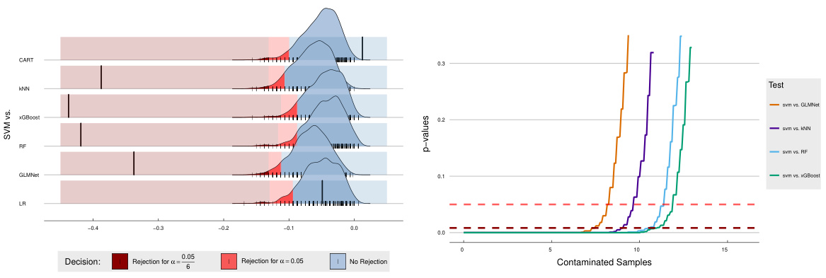
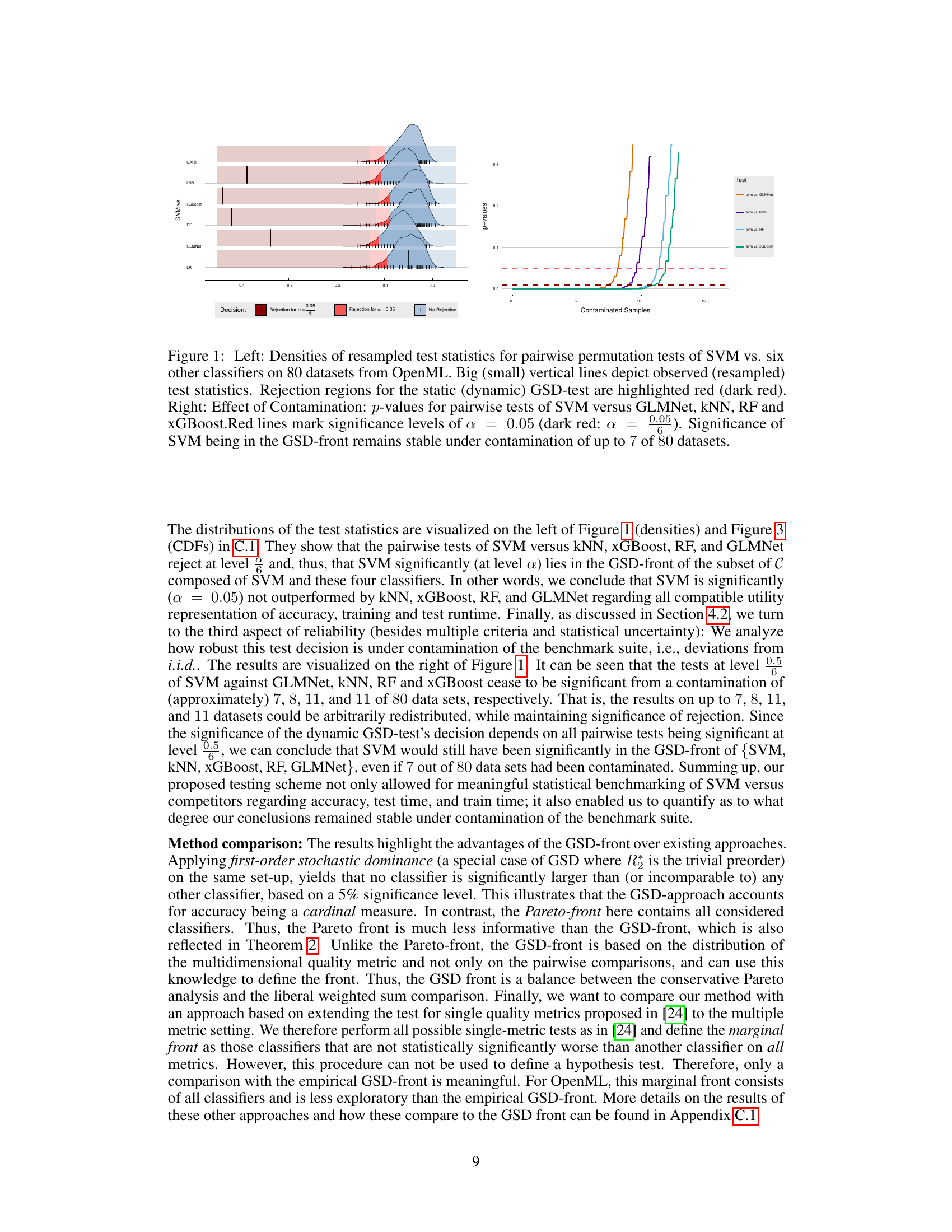
This figure shows the results of statistical testing to determine if SVM is in the GSD-front. The left panel displays density plots of resampled test statistics for pairwise comparisons of SVM against six other classifiers, using 80 datasets from OpenML. Vertical lines indicate observed and resampled test statistics; shaded regions highlight rejection areas for static and dynamic GSD tests. The right panel illustrates the robustness of the p-values to data contamination, showing how many contaminated samples are needed before significance is lost for each pairwise comparison.

This table presents the results of pairwise comparisons of seven algorithms (LR, RF, CART, SVM, xGBoost, GLMNet, kNN) using the Nemenyi post-hoc test following a Friedman test. The p-values indicate the statistical significance of differences in accuracy between algorithm pairs. Underlined p-values are less than 0.05, indicating a statistically significant difference in accuracy at the 5% significance level. The table shows which algorithms perform significantly better or worse than others in terms of prediction accuracy, based on the OpenML benchmark dataset. Note that this is just the accuracy metric, out of the three used in the OpenML experiment.

In-depth insights
#

GSD-Front Concept
#

The GSD-front, a novel concept in multicriteria classifier benchmarking, offers a powerful alternative to the traditional Pareto-front. Instead of solely identifying non-dominated classifiers, it leverages the principles of generalized stochastic dominance (GSD) to create a more refined and informative ranking. This approach acknowledges the inherent uncertainty in multidimensional quality metrics, addressing the challenge of comparing classifiers across multiple, potentially conflicting criteria. By incorporating both ordinal and cardinal information from different metrics, the GSD-front provides a more nuanced and discriminating comparison than methods that rely solely on component-wise dominance. The GSD-front’s key advantage lies in its ability to distinguish between classifiers that might be incomparable under Pareto analysis, offering a more efficient and insightful way to evaluate and rank classifiers based on their overall performance profiles. This concept is further strengthened by the introduction of consistent statistical estimators and robust testing procedures, enhancing its practical utility and reliability in real-world benchmarking scenarios.

Statistical Testing
#

The section on Statistical Testing is crucial for validating the claims made in the paper regarding the GSD-front. It addresses the statistical uncertainty inherent in using a limited benchmark suite to draw conclusions about a broader classifier population. Consistent statistical estimators are introduced to estimate the GSD-front from sample data. A significant contribution is the development of statistical tests to determine whether a new classifier belongs to the GSD-front, which adds practical value beyond simple Pareto-front comparisons. The discussion then extends to the important topic of robustness under non-i.i.d. (independently and identically distributed) sampling assumptions, a common weakness in benchmarking studies. This demonstrates a nuanced understanding of practical limitations and seeks to increase the reliability of the results. The methodology presented enhances the trustworthiness of multicriteria benchmarking, by incorporating statistical rigor. Both static and dynamic GSD-tests are proposed and analyzed. The authors show that these tests provide valid statistical evaluations while also possessing the consistency property (i.e. the reliability of the test increases with the size of the benchmark datasets). Ultimately, this rigorous statistical treatment strengthens the overall contribution of the paper and its applicability in practical classifier benchmarking.

Robustness Checks
#

Robustness checks in a research paper are crucial for establishing the reliability and generalizability of the findings. They assess how sensitive the results are to deviations from the assumptions made during the analysis. In the context of a machine learning study, robustness checks might involve evaluating the model’s performance on various data subsets, testing the impact of noise or outliers, and examining the model’s sensitivity to parameter choices. The goal is to demonstrate that the conclusions are not merely artifacts of specific assumptions or limited data characteristics, thus strengthening the confidence in the broader applicability of the research. A well-designed robustness analysis can significantly enhance the credibility and impact of a machine learning paper by showcasing the generalizability of its results. Furthermore, the choice of robustness tests themselves is crucial. Different robustness metrics may assess different aspects of the model’s stability, and a thorough evaluation might necessitate a comprehensive battery of tests.

Benchmarking Experiments
#

The heading ‘Benchmarking Experiments’ suggests a section dedicated to evaluating the performance of proposed methods against existing state-of-the-art techniques. A thoughtful analysis would delve into the datasets used, emphasizing their relevance and representativeness. The choice of evaluation metrics is crucial; the paper should justify the selected metrics and their suitability for the problem. Statistical significance testing is paramount to confirm that observed performance differences are not merely due to random chance. The section should also address the robustness of the results to various factors such as data set variability or different experimental setups. A comparative analysis of different methods is crucial to demonstrate the advantages and limitations of the proposed approach. A strong methodology section clearly outlining the experimental design, data handling, and validation techniques significantly enhances the credibility and impact of the presented findings. Ideally, the results would be presented in a clear and accessible manner, including tables and figures, to facilitate interpretation and comparison with previous work.

Future Research
#

The paper’s “Future Research” section suggests several promising avenues. Extending the GSD-front framework to other algorithm types beyond classifiers is crucial, opening doors to comparing optimizers or deep learning models across diverse metrics. Adapting the framework for regression-type analyses would enhance its applicability, especially with the inclusion of data set meta-properties. Stratifying GSD-analysis by relevant covariates within the data sets would allow for more nuanced situation-specific analyses, leading to potentially more informative results. The authors also mention investigating the impact of non-identically distributed (non-i.i.d.) data on the benchmark results and the robustness of statistical testing in such scenarios. Finally, research into the computational efficiency and scalability of the proposed methods, particularly for large-scale applications, is important to enhance practical usability.

More visual insights
#

More on figures

This figure shows a Hasse diagram representing the empirical generalized stochastic dominance (GSD) relations between seven classifiers on the OpenML benchmark dataset. A directed edge from one classifier to another indicates that the former empirically dominates the latter according to the GSD criterion. The classifiers included are: SVM, RF, CART, LR, GLMNet, xGBoost, and kNN. The shaded region highlights the classifiers that are not empirically dominated by any other classifier, representing the 0-empirical GSD-front. This visualization aids in understanding the relationships between the classifiers in terms of their performance across multiple quality metrics.

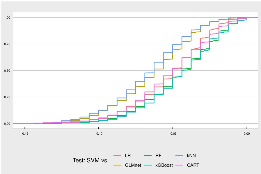
This figure shows the cumulative distribution functions (CDFs) of resampled test statistics for pairwise permutation tests comparing SVM against six other classifiers (LR, RF, kNN, GLMNet, xGBoost, and CART) on 80 datasets from OpenML. The observed test statistics are not shown in this graph but are listed in the caption. The distributions are compared visually, showing that the tests for SVM vs. xGBoost and GLMNet show a statistically significant difference from the other tests because their distributions are left-shifted.

This figure shows the empirical generalized stochastic dominance (GSD) relation for the Penn Machine Learning Benchmark (PMLB) dataset. The nodes represent different classifiers (CRE, SVM, RF, CART, GLMNet, kNN), and an edge from one node to another indicates that the first classifier empirically dominates the second according to the GSD criterion. The blue shaded area highlights the classifiers that constitute the 0-empirical GSD-front, meaning those classifiers that are not empirically dominated by any other classifier in the dataset. This visualization helps to understand the relative performance of different classifiers based on the GSD criterion.

This figure displays the density plots of the resampled test statistics from pairwise permutation tests comparing CRE against six other classifiers using the PMLB dataset. The vertical lines represent the observed test statistics, while the shaded regions indicate the rejection areas for both static and dynamic GSD tests at significance levels of α = 0.05 and α = 0.05/6. The results show that none of the pairwise tests reject the null hypothesis at either significance level, indicating that CRE does not statistically dominate any of the other classifiers considered.

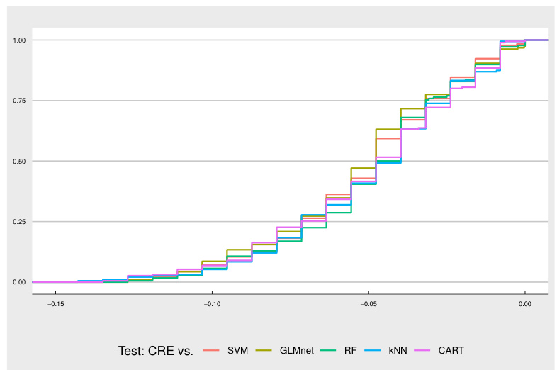
The figure displays the density plots of resampled test statistics for pairwise comparisons of a new classifier (CRE) against six other classifiers on 62 datasets from the PMLB benchmark. The vertical lines represent the observed test statistics from the actual experiment. The red-shaded areas indicate the rejection regions for the GSD test at significance levels α = 0.05. Since no observed statistic falls within the rejection region, the null hypothesis (that CRE is not significantly better than the compared classifiers) cannot be rejected at either significance level.

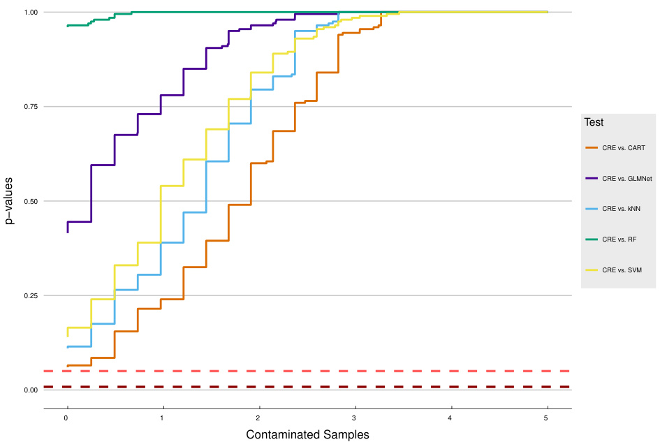
The figure shows the effect of data contamination on the p-values for pairwise tests comparing a new classifier (CRE) against five existing classifiers. The x-axis represents the number of contaminated samples, and the y-axis shows the p-values. The dotted red lines indicate the significance level (α = 0.05). Because none of the tests reject the null hypothesis at α=0.05 even without contamination, adding contaminated samples does not change this result. This demonstrates the robustness of the tests.