↗ OpenReview ↗ NeurIPS Proc. ↗ Chat
TL;DR#
Quadratic Unconstrained Binary Optimization (QUBO) is an NP-hard problem crucial in various fields, but existing learning-based solutions are computationally expensive due to their sequential decision-making process. Many existing learning-based approaches use deep reinforcement learning and model the solution as a Markov Decision Process (MDP), leading to high computational costs from repeated objective function evaluations.
This paper introduces the Value Classification Model (VCM), a novel neural solver that addresses these limitations. VCM uses a classification perspective, directly generating solutions instead of sequential decisions. It incorporates a Depth Value Network (DVN) to extract features and a Value Classification Network (VCN) to generate solutions. Training is done using a highly efficient Greedy-guided Self Trainer (GST) that doesn’t need optimal labels. Experimental results demonstrate VCM’s superior performance, achieving near-optimal solutions in milliseconds with remarkable generalization ability.
Key Takeaways#
Why does it matter?#
This paper is crucial for researchers in combinatorial optimization and machine learning. It presents a novel and highly efficient method for solving a notoriously difficult problem, advancing the field and opening new avenues of research. The classification-based approach offers significant advantages over traditional sequential methods, demonstrating improved performance and scalability. This work is particularly important given the growing interest in applying machine learning techniques to solve complex optimization problems.
Visual Insights#
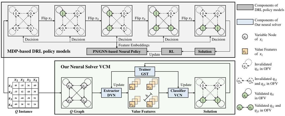
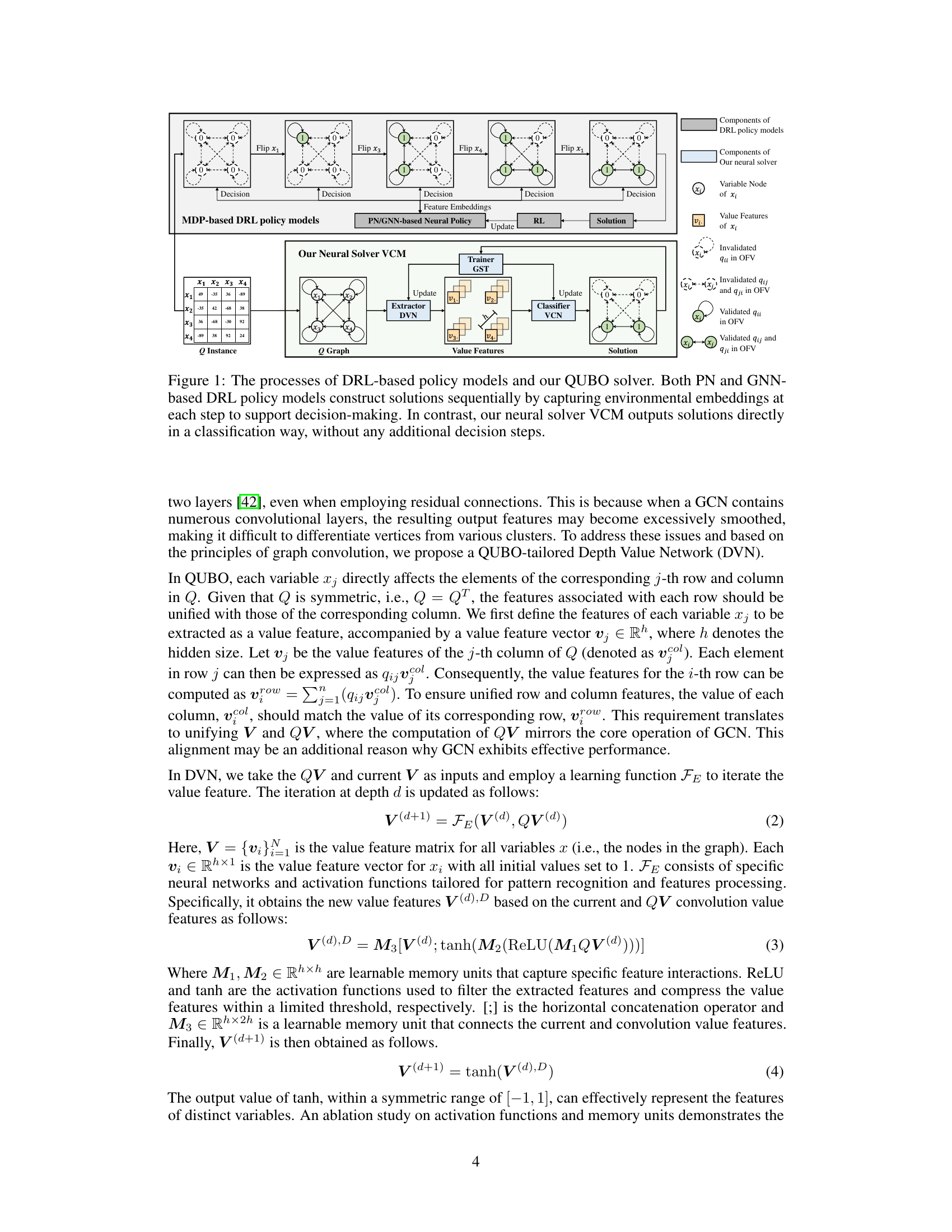
This figure compares the solution processes of traditional DRL-based methods (PN and GNN) and the proposed Value Classification Model (VCM) for solving the Quadratic Unconstrained Binary Optimization (QUBO) problem. DRL-based methods solve QUBO sequentially, making decisions one variable at a time based on features extracted at each step. In contrast, VCM directly generates a complete solution by classifying the values of all variables simultaneously. The figure highlights the difference in computational complexity and efficiency between the approaches.
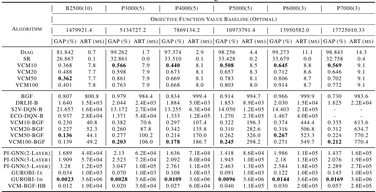
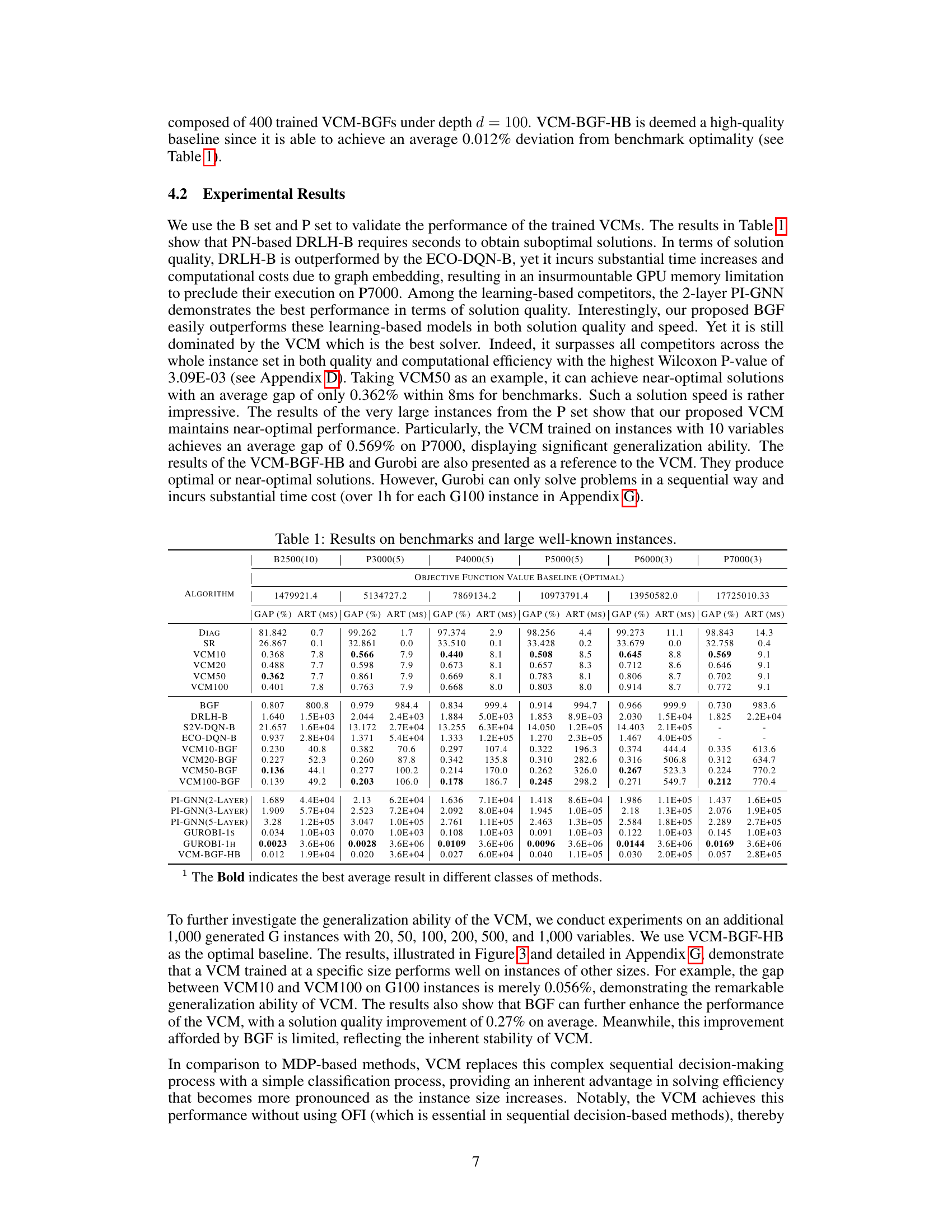
This table presents the performance comparison of the proposed VCM model against various state-of-the-art methods and traditional solvers on benchmark instances (B2500) and very large instances (P3000-P7000). The comparison is based on two key metrics: the optimality gap (GAP) and the average running time (ART). The table allows readers to easily assess VCM’s efficiency and solution quality compared to existing techniques. The results show that VCM outperforms its competitors in terms of both solution quality and computational speed, achieving near-optimal results in milliseconds even for very large problem instances.
In-depth insights#
QUBO’s Challenges#
Quadratic Unconstrained Binary Optimization (QUBO) presents significant computational challenges due to its NP-hard nature. Existing approaches, often sequential decision-making processes based on Markov Decision Processes (MDPs) and techniques like Pointer Networks (PNs) or Graph Neural Networks (GNNs), suffer from high computational complexity and limited scalability. PN-based methods struggle with variable-sized input matrices, while GNNs encounter memory and storage bottlenecks as problem size increases. Moreover, the repeated evaluation of the objective function inherent in MDP-based methods adds to the computational burden, especially for large-scale instances. Addressing these limitations requires innovative techniques that move beyond the sequential decision paradigm of existing methods and avoid repeated computations, potentially through parallel processing or clever approximation strategies. Developing efficient and scalable algorithms for QUBO remains a crucial area of research with significant implications for various fields.
VCM Architecture#
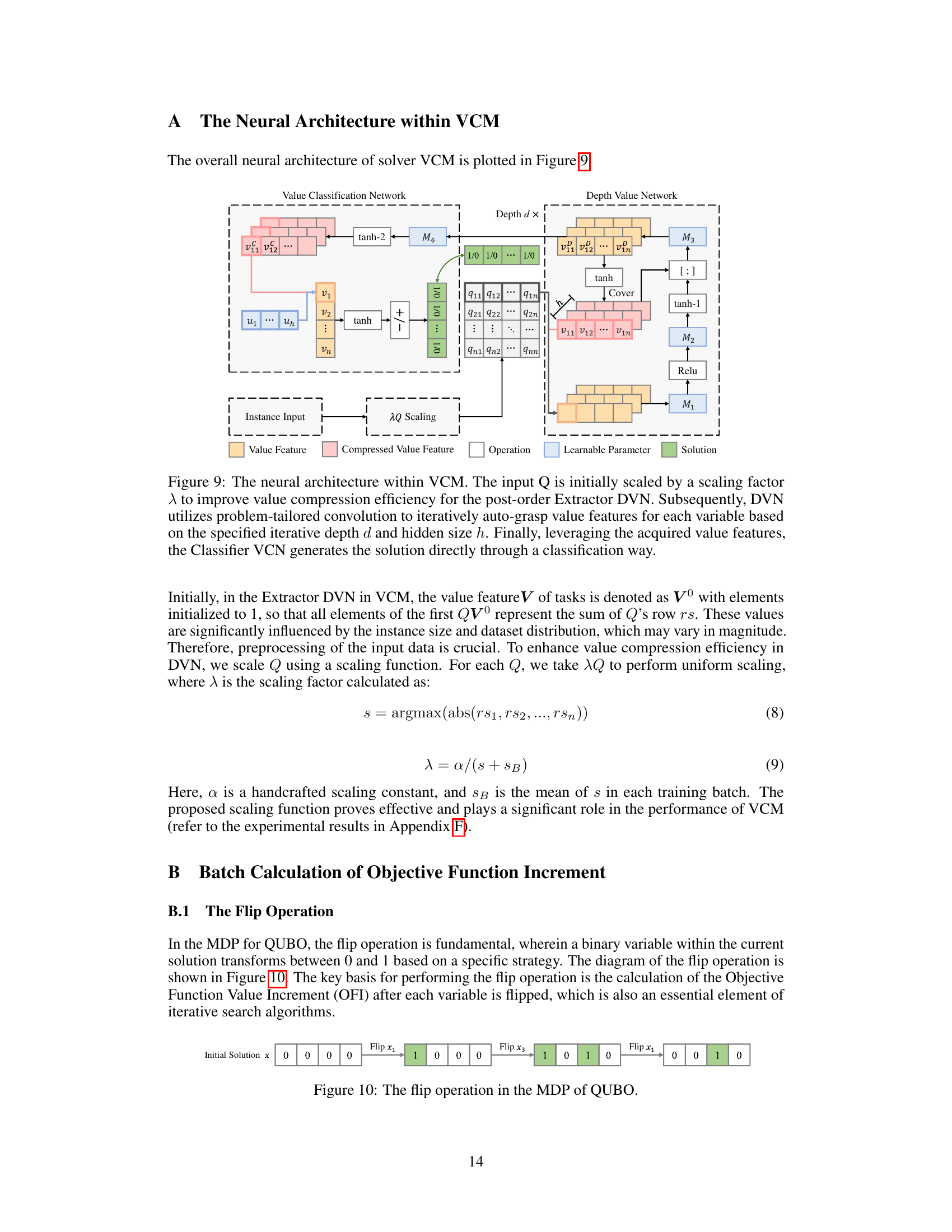
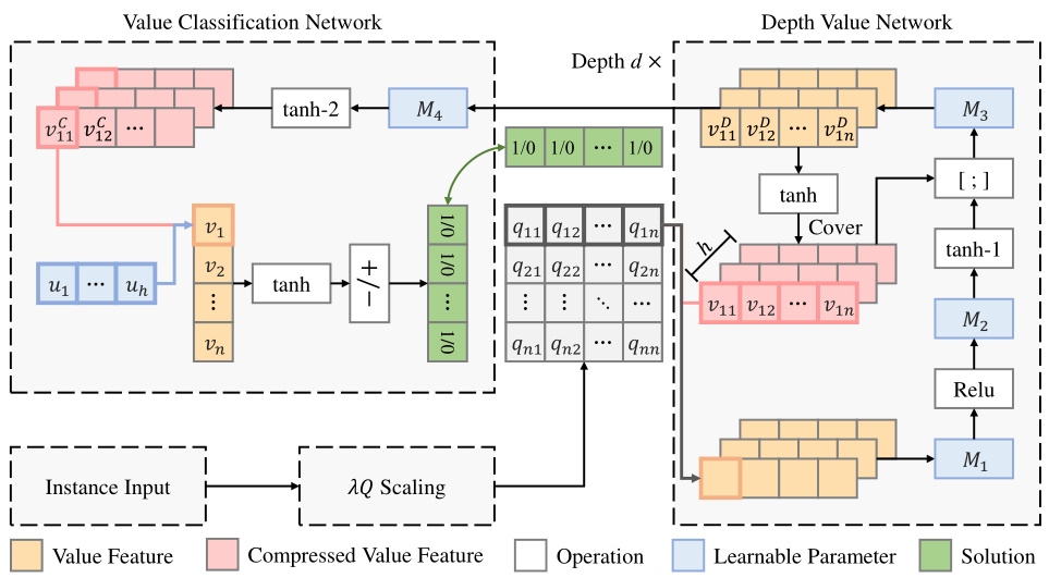
The Value Classification Model (VCM) architecture is a novel approach to solving Quadratic Unconstrained Binary Optimization (QUBO) problems. It departs from traditional sequential methods by framing QUBO as a classification problem. Central to VCM is the Depth Value Network (DVN), which leverages graph convolutional operations to efficiently extract value features from the input Q matrix. This leverages the inherent symmetry in Q, avoiding the computational burden of sequential decision-making inherent in Markov Decision Process (MDP) based approaches. The extracted features are then fed into the Value Classification Network (VCN), which directly generates the solution vector x. The training process uses a Greedy-guided Self Trainer (GST), eliminating the need for pre-labeled optimal solutions. The GST guides the training with near-optimal solutions generated by a greedy heuristic, drastically improving efficiency. This unique combination of DVN, VCN, and GST allows VCM to achieve near-optimal solutions with remarkable speed and generalization capabilities.
Greedy Self-Train#
A ‘Greedy Self-Train’ approach for training a model to solve Quadratic Unconstrained Binary Optimization (QUBO) problems is a compelling idea. It cleverly sidesteps the need for labeled data, a major hurdle in QUBO problem training, by using a greedy heuristic to generate pseudo-labels. This is particularly efficient because it avoids the computationally expensive process of obtaining optimal solutions, which is often infeasible for large problems. The ‘greedy’ aspect ensures a fast iterative improvement process while the ‘self-train’ aspect bootstraps the learning process. This method’s efficacy hinges on the quality of the pseudo-labels generated by the greedy algorithm. A good greedy algorithm should produce solutions close to optimal, allowing the model to learn effectively. However, if the greedy heuristic is poorly designed, the pseudo-labels could be misleading, potentially hindering model learning. The success of this method thus relies on a delicate balance between greedy algorithm efficiency and label quality. A thorough evaluation comparing the performance of this method against alternative training approaches on various benchmarks is crucial to assess its overall effectiveness and identify potential limitations.
DVN Depth Impact#
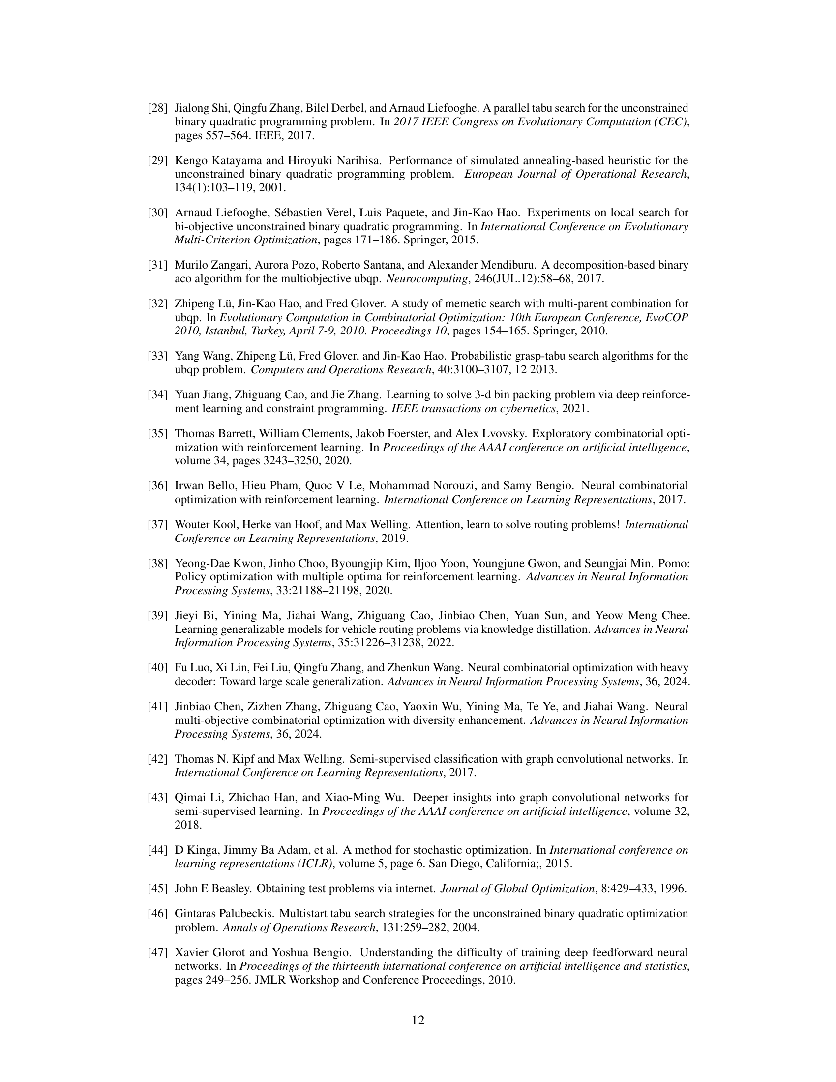
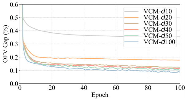
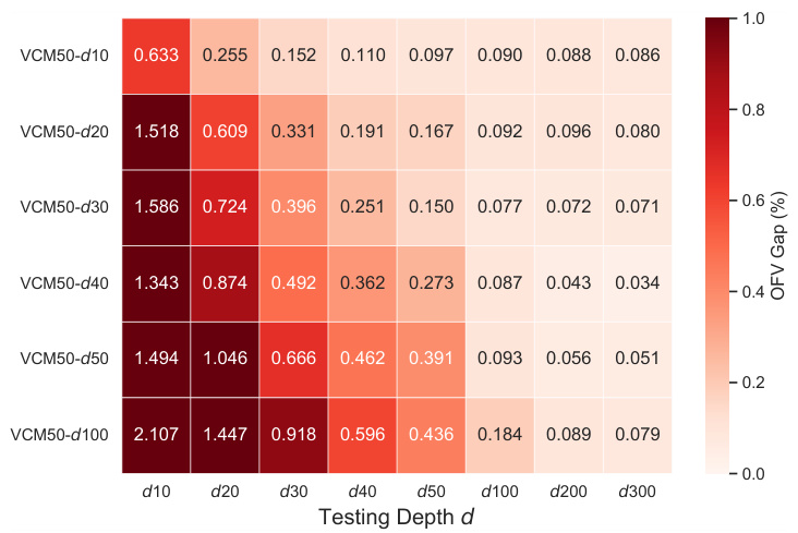
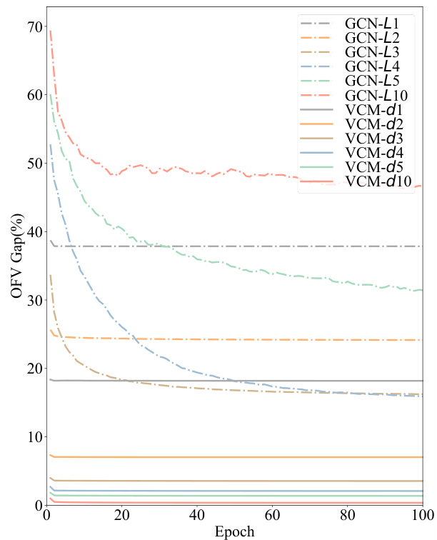
The DVN (Depth Value Network) depth significantly impacts the performance of the Value Classification Model (VCM). Increasing the DVN depth improves the quality of extracted value features, leading to a steady enhancement in VCM’s solution accuracy. This improvement is particularly notable when the testing depth surpasses the training depth, demonstrating that the model continues to learn and refine its feature extraction even beyond its initial training. This characteristic distinguishes VCM from GCNs, which exhibit performance degradation with increased depth. The computational cost of increasing depth is linear, making it a practical trade-off for higher accuracy. The ability of VCM to benefit from increased testing depth without retraining highlights its efficiency and adaptability, suggesting that a properly trained VCM can steadily find better solutions simply by increasing the testing depth and offering potential cost savings compared to retraining the entire model.
Future of VCM#
The “Future of VCM” section would explore avenues for enhancing the model’s capabilities and addressing its limitations. Optimality improvements could focus on refining the value classification network (VCN) architecture or integrating more sophisticated methods for handling value features from the depth value network (DVN). Expanding applicability to other combinatorial optimization problems would involve testing VCM’s effectiveness on diverse problem structures and adapting the feature extraction mechanisms accordingly. Research into more efficient training methods is crucial; exploring techniques beyond the greedy-guided self-trainer (GST) could significantly reduce training time and improve generalization. Finally, exploring the integration of VCM with other methods, such as heuristic algorithms, could further boost performance and robustness, leading to a more versatile and powerful solver for QUBO and related problems.
More visual insights#
More on figures

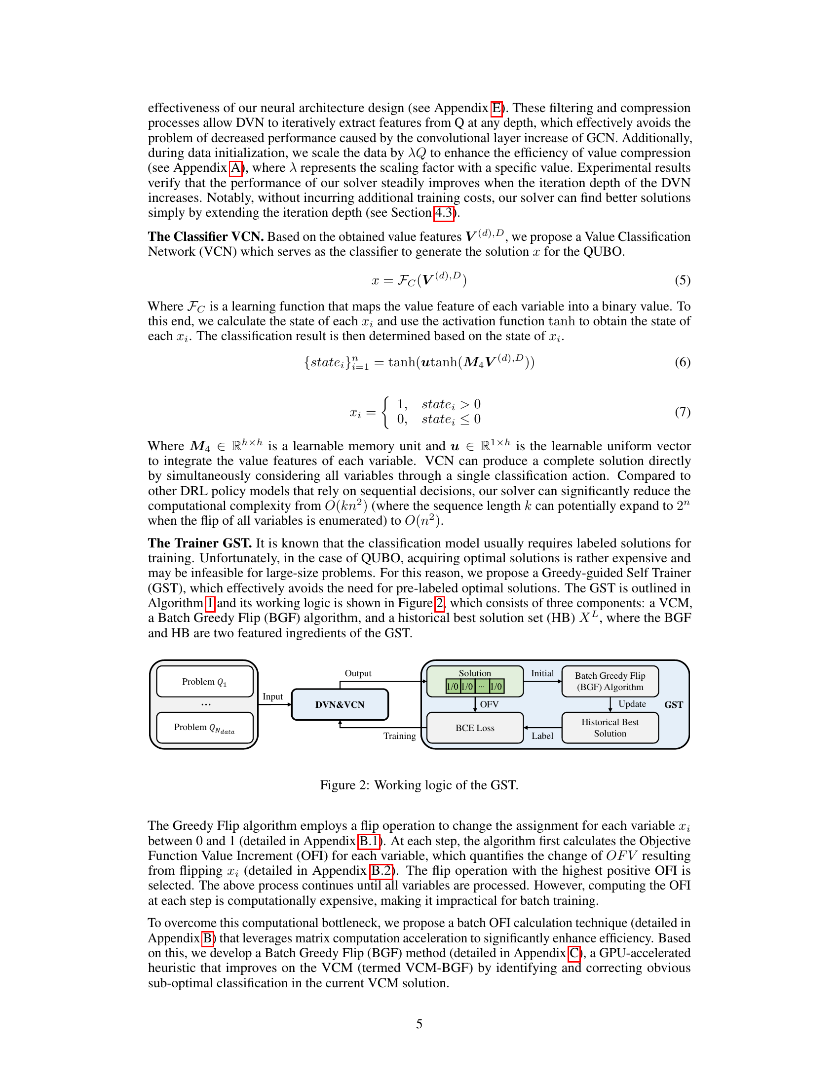
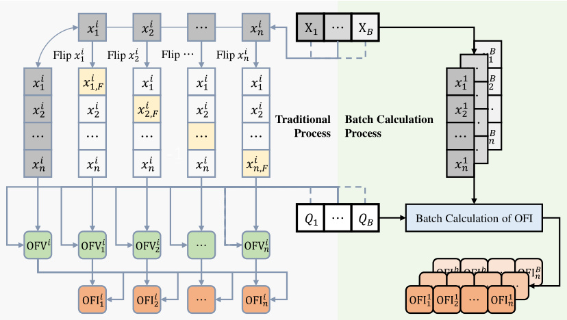
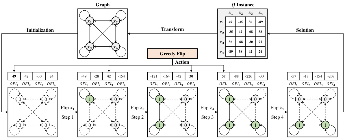
The figure illustrates the workflow of the Greedy-guided Self Trainer (GST). It starts with input problem instances (Q1 to QNdata). These are fed into the Depth Value Network (DVN) and Value Classification Network (VCN) which produce an initial solution. This solution’s objective function value (OFV) is calculated. The Batch Greedy Flip (BGF) algorithm then iteratively refines the solution. The OFV and the refined solution are used to calculate a Binary Cross Entropy (BCE) Loss, and this loss is used to update the DVN and VCN weights in a training loop. The best solution obtained across all training epochs is stored as a Historical Best Solution and fed back into the next training cycle. The entire process is self-supervised, meaning it learns without needing pre-labeled optimal solutions.

This figure compares the solution processes of traditional Deep Reinforcement Learning (DRL) models using Pointer Networks (PN) or Graph Neural Networks (GNN) with the proposed Value Classification Model (VCM). DRL methods sequentially build solutions by making decisions based on learned embeddings at each step. In contrast, VCM directly generates complete solutions through a classification approach.

This figure compares the solution processes of traditional DRL-based methods (PN and GNN) and the proposed VCM for solving the QUBO problem. DRL methods build solutions step-by-step, making sequential decisions based on environmental embeddings. In contrast, VCM directly generates a complete solution through a single classification process, significantly improving efficiency.
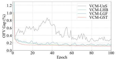
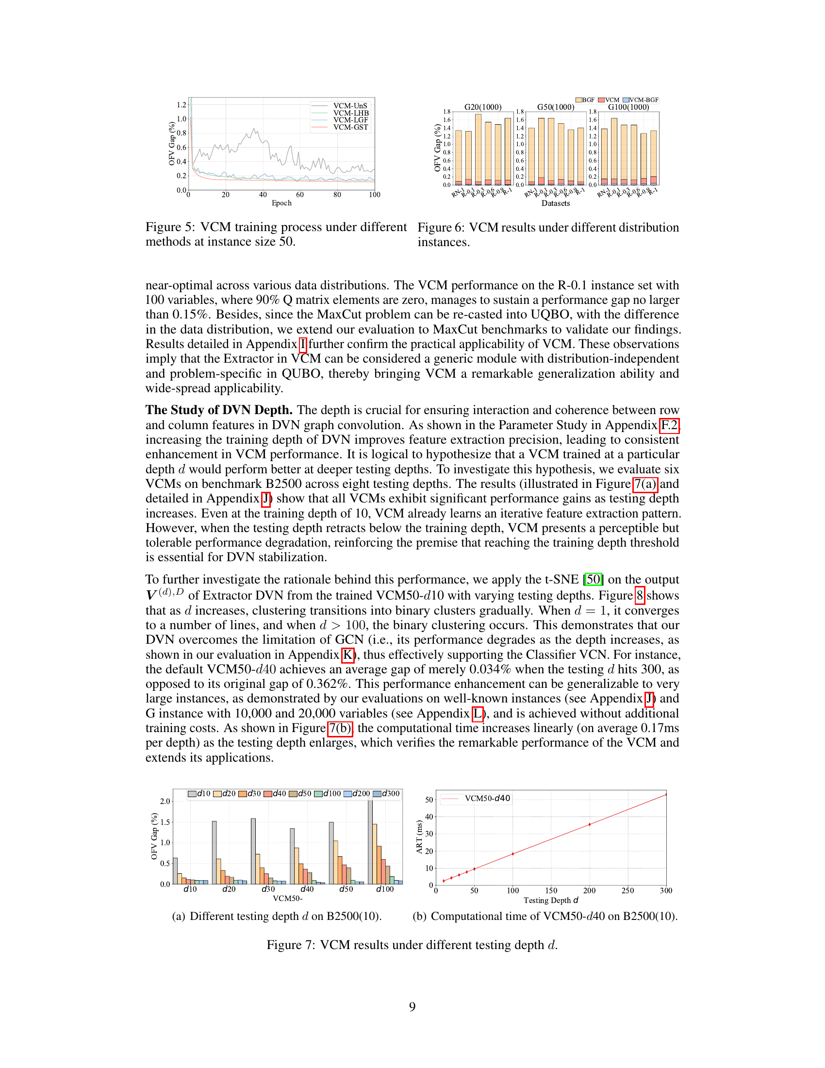
This figure shows the training curves of various training methods for the VCM model at instance size 50. The methods compared include an unsupervised training method (UnS), supervised learning with optimal labels (LHB), supervised learning with labels generated by the current VCM-BGF (LGF), and the proposed Greedy-guided Self Trainer (GST). The figure demonstrates that the GST outperforms other methods in both efficiency and stability, achieving similar performance to LHB while requiring fewer epochs and maintaining consistent performance compared to the fluctuating results of UnS and LGF.
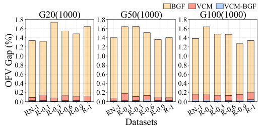
This figure shows the generalization ability of the Value Classification Model (VCM) and its enhanced version VCM-BGF across different dataset sizes. The x-axis represents the different datasets used, and the y-axis shows the average OFV gap (%). The bars represent the performance of VCM and VCM-BGF on these datasets. The figure demonstrates that even when trained on small datasets, VCM and VCM-BGF maintain good performance on larger datasets. The results indicate remarkable generalization ability.

This figure compares the solution processes of traditional deep reinforcement learning (DRL) based methods, specifically those using Pointer Networks (PN) or Graph Neural Networks (GNN), with the proposed Value Classification Model (VCM). DRL methods solve QUBO problems sequentially, making decisions step-by-step and updating the solution iteratively. In contrast, VCM directly generates the solution in one step via a classification approach.
This figure compares the solution processes of traditional Deep Reinforcement Learning (DRL) models using Pointer Networks (PN) or Graph Neural Networks (GNN) with the proposed Value Classification Model (VCM). DRL methods solve the Quadratic Unconstrained Binary Optimization (QUBO) problem sequentially, making a series of decisions to flip individual binary variables. Each decision requires evaluating the impact of the flip on the objective function. VCM, in contrast, solves QUBO in a single classification step, directly predicting the optimal values of all variables simultaneously without sequential decision-making.

This figure compares the solution processes of traditional Deep Reinforcement Learning (DRL) methods and the proposed Value Classification Model (VCM). DRL methods, using Pointer Networks (PN) or Graph Neural Networks (GNNs), iteratively build solutions by making sequential decisions based on learned embeddings. In contrast, VCM directly generates the entire solution in one step via classification, significantly improving efficiency.
This figure compares the processes of traditional DRL-based methods (PN and GNN) and the proposed Value Classification Model (VCM) for solving the QUBO problem. DRL methods solve QUBO sequentially, making decisions step-by-step, evaluating the impact of each decision on the objective function. In contrast, the VCM generates a complete solution directly using a classification approach, significantly improving computational efficiency.
This figure compares the solution processes of traditional Deep Reinforcement Learning (DRL) methods (using Pointer Networks (PN) or Graph Neural Networks (GNN)) and the proposed Value Classification Model (VCM). DRL methods solve the Quadratic Unconstrained Binary Optimization (QUBO) problem sequentially, making decisions step-by-step based on embeddings of problem data. In contrast, the VCM directly generates a complete solution through a classification process, significantly improving efficiency.
This figure compares the solution processes of traditional Deep Reinforcement Learning (DRL) models (PN and GNN-based) with the proposed Value Classification Model (VCM). DRL models solve the QUBO problem sequentially, making decisions step-by-step based on embedding features. In contrast, the VCM solves the problem directly in a classification way, providing all solution variables simultaneously. The figure highlights the fundamental difference in efficiency and approach between these methods.
This figure compares the solution processes of traditional deep reinforcement learning (DRL) based models for solving Quadratic Unconstrained Binary Optimization (QUBO) problems with the proposed Value Classification Model (VCM). DRL models, using either Pointer Networks (PN) or Graph Neural Networks (GNN), build solutions step-by-step, making decisions at each step based on learned embeddings. In contrast, VCM directly generates a complete solution via a classification approach. The figure visually illustrates this difference in the solution process, emphasizing VCM’s efficiency and directness.
This figure compares the processes of traditional Deep Reinforcement Learning (DRL) based methods (using Pointer Networks or Graph Neural Networks) and the proposed Value Classification Model (VCM) for solving the Quadratic Unconstrained Binary Optimization (QUBO) problem. DRL methods solve QUBO sequentially, making decisions one variable at a time, while VCM solves it directly through a single classification step, significantly improving efficiency.
This figure compares the solution processes of traditional deep reinforcement learning (DRL) models, which use pointer networks (PN) or graph neural networks (GNN), and the proposed Value Classification Model (VCM). DRL models solve QUBO problems sequentially by making decisions at each step, which are guided by learned embeddings of the problem’s structure. This sequential process can be computationally expensive. In contrast, VCM directly generates the full solution in a single classification step, which significantly increases computational efficiency.
This figure compares the solution processes of traditional Deep Reinforcement Learning (DRL) based methods (PN and GNN) and the proposed Value Classification Model (VCM). DRL methods solve QUBO problems sequentially, making decisions step-by-step. In contrast, VCM solves the problem by directly generating a classification-based solution in a single step, significantly improving efficiency.

This figure compares the solution processes of traditional Deep Reinforcement Learning (DRL) models (PN and GNN-based) with the proposed Value Classification Model (VCM). DRL methods solve the problem sequentially by making decisions at each step, evaluating the impact of each action on the objective function. In contrast, VCM directly generates a complete solution through a classification process, which avoids the repeated evaluations of objective function values that are computationally costly in the DRL approaches. The figure highlights the different components and workflows of the two types of methods, illustrating VCM’s efficiency and innovation.
This figure compares the solution processes of traditional Deep Reinforcement Learning (DRL) based models and the proposed Value Classification Model (VCM) for solving Quadratic Unconstrained Binary Optimization (QUBO) problems. DRL methods, using either Pointer Networks (PN) or Graph Neural Networks (GNN), build solutions step-by-step, making sequential decisions at each step based on learned embeddings of the problem’s state. In contrast, the VCM directly generates a complete solution through a single classification step, eliminating the iterative decision-making process of DRL approaches. The visual representation highlights the key difference in approach, showing the sequential steps of DRL models versus the direct solution output of VCM.
The figure illustrates the working mechanism of the Greedy-guided Self Trainer (GST). It shows how the GST uses a VCM (Value Classification Model), a BGF (Batch Greedy Flip) algorithm, and an HB (Historical Best Solution) set to iteratively improve solutions. The VCM generates an initial solution, which is then refined by the BGF algorithm to find better solutions. These improved solutions are then stored in the HB set, which provides labels for the next training iteration. This iterative process continues until satisfactory performance is achieved.
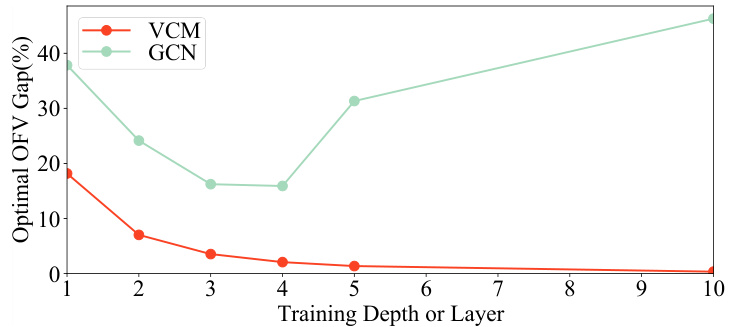
This figure compares the performance of GCN and VCM in terms of the optimal OFV gap achieved during training. The x-axis represents the training depth (for VCM) or the number of layers (for GCN), while the y-axis shows the optimal OFV gap (%). The graph illustrates that VCM demonstrates significantly better performance and stability compared to GCN as the training depth/number of layers increases. The optimal OFV gap for VCM remains consistently low, while it increases significantly for GCN, highlighting VCM’s advantage in this aspect.
More on tables

This table presents the performance comparison of the proposed Value Classification Model (VCM) against various state-of-the-art algorithms on benchmark instances (B2500) and well-known instances (P3000, P4000, P5000, P6000, P7000). The comparison is based on two key metrics: the optimality gap (GAP) and the average running time (ART). The results showcase VCM’s superior performance in terms of both solution quality and computational efficiency across different instance sizes. It highlights VCM’s remarkable generalization ability, achieving near-optimal solutions within milliseconds even on very large instances.

This table presents the performance comparison of different algorithms on benchmark datasets (B) and well-known instances (P). The algorithms include various heuristic methods, learning-based sequential decision models, and the proposed VCM model. For each algorithm, the table reports the average optimality gap (percentage difference from the optimal solution) and average runtime (in milliseconds). The results show that the VCM model significantly outperforms other methods in terms of both solution quality and computational efficiency. Notably, the VCM model trained on smaller instances exhibits remarkable generalization ability when applied to larger instances.
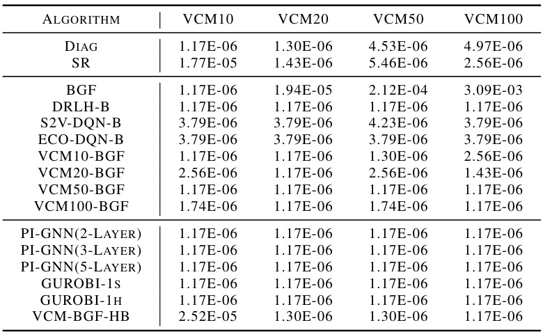
This table presents the performance comparison of various algorithms, including the proposed VCM and several baselines (e.g., Gurobi, DRLH, PI-GNN) on benchmark datasets (B) and large-scale instances (P). It shows the optimality gap (%) and average running time (ms) achieved by each method, highlighting the superior performance of the VCM in terms of both solution quality and computational efficiency.
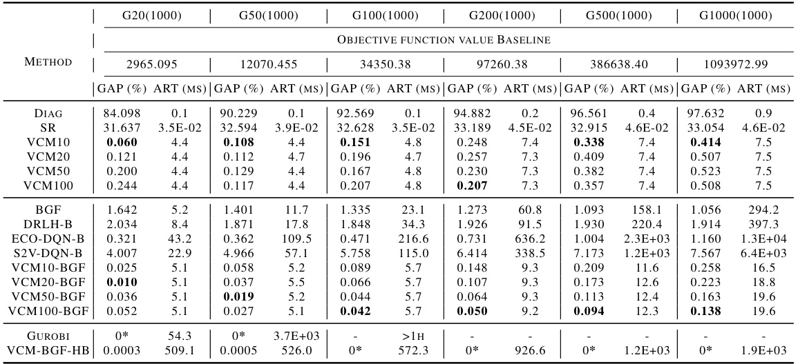
This table presents the performance comparison of various algorithms (DIAG, SR, VCM variants, BGF, DRLH-B, S2V-DQN-B, ECO-DQN-B, PI-GNN variants, Gurobi with 1-second and 1-hour time limits, VCM-BGF-HB) on benchmark datasets (B2500(10)) and well-known instances (P3000(5), P4000(5), P5000(5), P6000(3), P7000(3)). The comparison metrics are the optimality gap (%) and the average running time in milliseconds (ms). It showcases the superior performance of the proposed VCM in terms of both solution quality and computational efficiency.
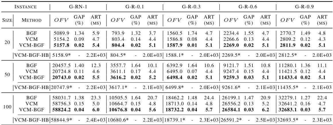
This table presents the performance comparison of various algorithms (DIAG, SR, VCM variations, BGF, DRLH-B, S2V-DQN-B, ECO-DQN-B, PI-GNN variations, Gurobi) on benchmark datasets (B2500(10)) and large-scale, well-known instances (P sets). The comparison is done using the OFV gap (%) (difference from the optimal OFV) and average running time (ART in milliseconds). The results demonstrate the superior performance of the proposed VCM in terms of both solution quality and efficiency.

This table presents the results of the proposed Value Classification Model (VCM) and other methods on benchmark and well-known instances. For each dataset, it shows the average optimality gap (GAP) and the average running time (ART). It allows to compare VCM against a range of baselines including exact methods (Gurobi), heuristic methods (Diag, SR, BGF), learning-based sequential decision methods (DRLH-B, S2V-DQN-B, ECO-DQN-B), and a physics-inspired neural solver (PI-GNN). The results highlight VCM’s superior performance in terms of both solution quality and speed.

This table presents the performance comparison of various algorithms on benchmark instances (B) and well-known instances (P) of different sizes. The algorithms are compared based on the average optimality gap (percentage deviation from the optimal solution) and the average running time (in milliseconds). The table shows the performance of various heuristic methods, learning-based methods (including the proposed VCM and its variants), and an exact solver (Gurobi). The results highlight the VCM’s superior performance in terms of both solution quality and computational efficiency, especially for larger instances.

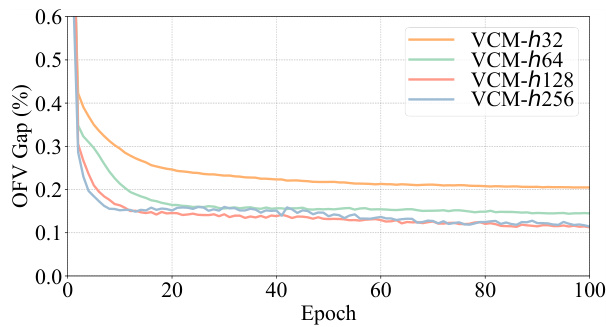
This table presents the results of the DVN depth experiment. It shows the average gap and average running time (ART) on benchmarks B2500(10) for various testing depths (10, 20, 30, 40, 50, 100, 200, and 300) and training depths (10, 20, 30, 40, 50, and 100). The results demonstrate the impact of increasing testing and training depths on the model’s performance.

This table presents the performance comparison of various algorithms (including the proposed VCM and its variants, baseline methods, and state-of-the-art learning-based approaches) on benchmark and well-known QUBO instances. The metrics used for evaluation are the optimality gap (percentage deviation from the optimal solution) and the average running time (in milliseconds). The table showcases the superior performance of the VCM in terms of both solution quality and computational efficiency across different problem sizes.

This table presents the performance comparison of different algorithms on benchmark datasets (B) and well-known instances (P). The results are compared in terms of the optimality gap (percentage difference from the optimal solution) and the average running time (in milliseconds). The algorithms compared include various heuristic methods, learning-based sequential decision models and the proposed VCM at different training depths. The optimal solution values are provided as a baseline for comparison.
Full paper#
