↗ OpenReview ↗ NeurIPS Proc. ↗ Chat
TL;DR#
Many real-world problems can be modeled using probabilistic models. However, one of the fundamental tasks in probabilistic modeling, namely the Most Probable Explanation (MPE) query, is computationally expensive and challenging to solve, particularly for large, complex models. Existing methods either lack accuracy or are computationally infeasible for large-scale applications.
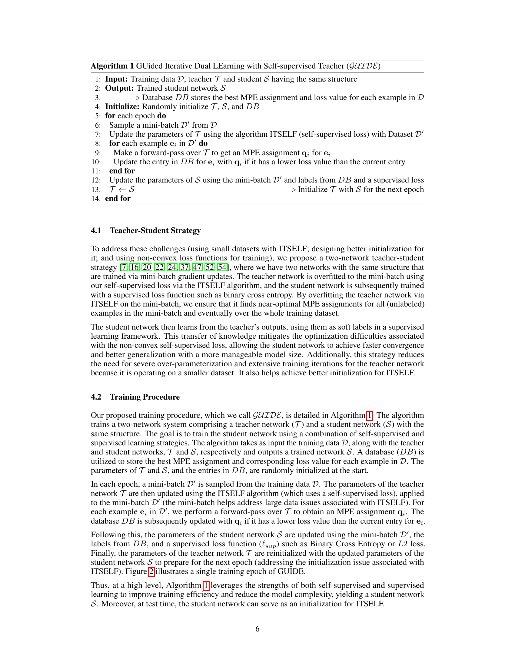
This research proposes a novel neural-network based approach called GUIDE to efficiently compute the MPE. The core idea is to train a neural network to directly answer MPE queries instead of relying on traditional inference algorithms. The approach incorporates inference-time optimization and a teacher-student framework to improve solution quality and speed. Experiments on various datasets and probabilistic models demonstrate the method’s superior performance compared to existing baselines, showcasing both higher accuracy and faster inference times.
Key Takeaways#
Why does it matter?#
This paper is crucial for researchers working on probabilistic models because it provides a novel and efficient neural network approach for solving the NP-hard MPE query problem. This has wide-ranging implications for various applications, and the proposed method’s scalability and efficacy make it particularly relevant to current research trends focusing on large-scale probabilistic modeling.
Visual Insights#

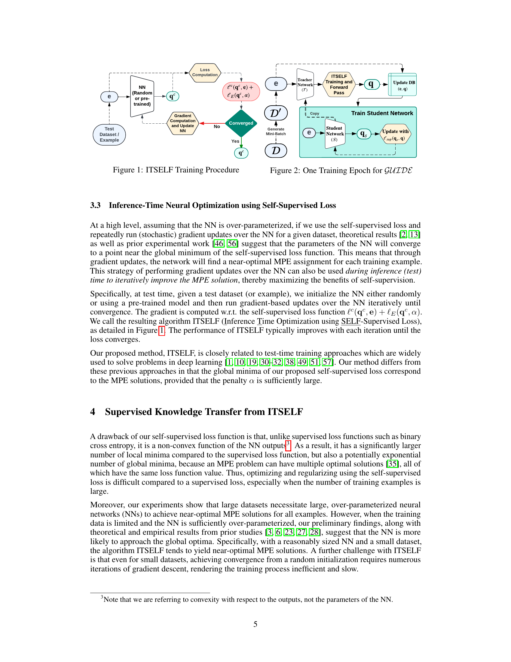
This figure illustrates the iterative process of the Inference Time Self Supervised Training (ITSELF) algorithm. Starting with a random or pre-trained neural network, the algorithm iteratively refines the MPE solution during the inference process. The NN receives evidence (e) as input and outputs a continuous MPE assignment (q^c). The self-supervised loss function, lc(q^c, e) + le(q^c, α), is computed. Gradient descent then updates the network parameters. This process repeats until convergence, yielding a refined MPE assignment (q^f).
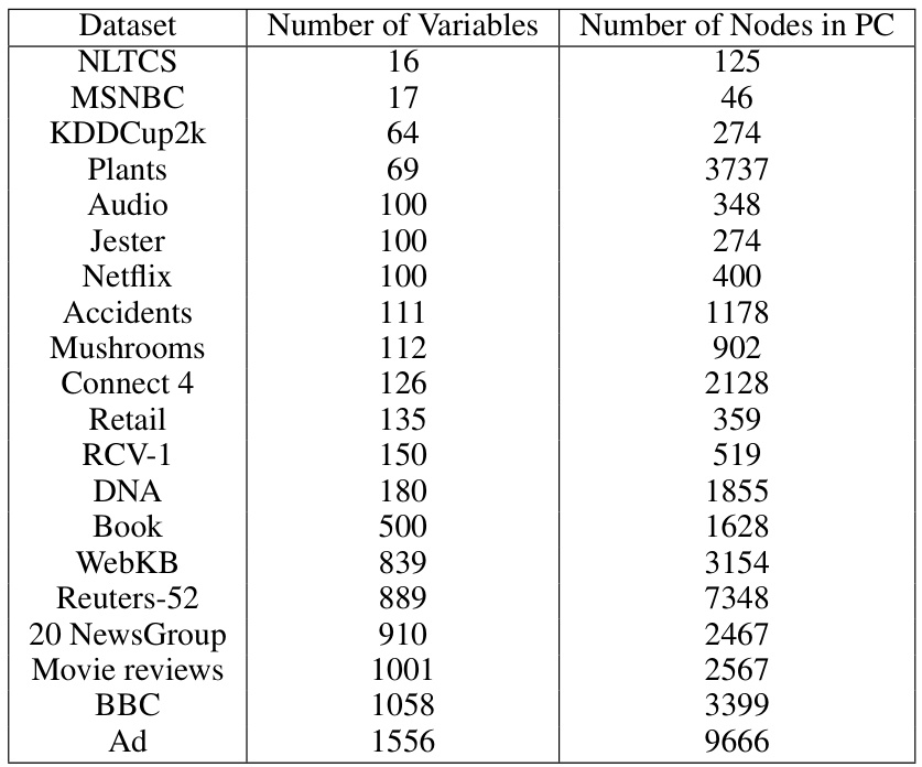
This table summarizes the 20 benchmark datasets used in the paper for evaluating probabilistic circuits (PCs) and neural autoregressive models (NAMs). For each dataset, it shows the number of variables and the number of nodes in the corresponding PC. The datasets range in size from relatively small (e.g., NLTCS with 16 variables) to very large (e.g., Ad with 1556 variables), reflecting a broad spectrum of complexity levels.
In-depth insights#
Neural MPE Inference#
The concept of ‘Neural MPE Inference’ signifies a paradigm shift in tackling the computationally complex Most Probable Explanation (MPE) problem within probabilistic models. Traditional approaches often struggle with the NP-hard nature of MPE, especially for large-scale models. Neural methods offer a compelling alternative, leveraging the power of neural networks to learn an efficient approximation of the MPE solution. This approach involves training a neural network to directly output the most probable explanation given evidence. Key advantages include speed and scalability, outperforming traditional inference algorithms on various datasets and model types. However, challenges remain, such as the potential for overfitting and the non-convexity of the loss function. Advanced techniques like self-supervised learning and teacher-student frameworks aim to mitigate these issues and improve the quality and efficiency of the inferred MPE solutions. Future research directions could focus on addressing the limitations of neural approaches, enhancing robustness, expanding to broader classes of probabilistic models, and improving explainability.
Self-Supervised Loss#
A self-supervised learning approach for the Most Probable Explanation (MPE) task in probabilistic models is presented. The core idea revolves around distilling all MPE queries into a neural network, thus eliminating the need for traditional inference algorithms. A crucial aspect is the design of a self-supervised loss function. This function guides the training process without the need for labeled data, making the approach more practical and scalable. The function’s differentiability and tractability are vital for efficient training, enabling gradient-based updates. Its design leverages the properties of the probabilistic models, making the loss function computationally manageable. In essence, the loss function is engineered to minimize the negative log-likelihood and achieve near-optimal MPE solutions. By refining the loss with techniques like an entropy-based penalty, the quality of the solutions is iteratively improved during inference. This self-supervised approach represents a significant step towards more efficient and scalable MPE inference, especially for larger, complex models where traditional methods fall short.
ITSELF Optimization#
The concept of “ITSELF Optimization” presented in the paper suggests an iterative, self-improving approach to solving the Most Probable Explanation (MPE) problem. ITSELF leverages a self-supervised neural network, trained to find MPE solutions, but rather than simply querying the network once, it iteratively refines its solution during the inference process. This refinement is achieved using gradient descent (backpropagation) on a self-supervised loss function. The iterative process allows for continual improvement of the MPE solution estimate, effectively providing an anytime algorithm where accuracy increases with computation time. The method is particularly useful when exact inference is computationally infeasible, as the continuous improvement towards an optimal solution remains possible even without prior knowledge of query variables. This iterative approach contrasts with traditional single-pass methods, offering the potential for significantly improved accuracy. The key innovation lies in using self-supervision to refine the network’s parameters during inference, offering an elegant and computationally efficient method for approximate MPE inference in large probabilistic models.
Teacher-Student Model#
Teacher-student models offer a powerful paradigm for improving the efficiency and effectiveness of complex machine learning tasks. In the context of this research paper, the teacher network, trained using a self-supervised loss function, learns to solve MPE queries directly from the underlying probabilistic model. This process, while computationally expensive, generates high-quality MPE solutions, which serve as a training dataset for the student network. The student network, trained using supervised learning, learns to approximate the teacher’s performance with significantly reduced computational cost, thus enabling faster and more efficient inference for arbitrary MPE queries. The key advantage lies in knowledge transfer: the teacher provides a strong initial estimate that helps the student to quickly converge to near-optimal solutions. This significantly reduces the need for extensive training iterations in the student model, thereby enhancing overall efficiency and scaling capabilities. The teacher-student framework addresses the challenges posed by self-supervised learning: specifically, overfitting and convergence difficulties associated with non-convex loss functions. By leveraging supervised learning, the student network gains regularization and avoids many of the pitfalls common to solely self-supervised approaches. The result is a scalable and accurate approach to answering MPE queries in various probabilistic models. The methodology’s success hinges on the ability of the teacher to distill the complexities of the probabilistic model into a representation readily learnable by the student.
Future Research#
The authors propose several promising avenues for future work, primarily focusing on enhancing the model’s capabilities and expanding its applicability. Extending the approach to handle complex queries with constraints is a key area, moving beyond the current any-MPE framework to address more nuanced real-world problems. Another important direction involves improving training by incorporating multiple probabilistic models, potentially leading to more robust and accurate inference. This suggests a move towards a more holistic and integrated approach to probabilistic modeling. Finally, the authors highlight the need for advanced encoding strategies, more sophisticated neural architectures, and exploring different loss functions to potentially unlock even greater efficiency and scalability. These improvements would solidify the model’s practical effectiveness and broaden its use across a wider range of probabilistic problems.
More visual insights#
More on figures
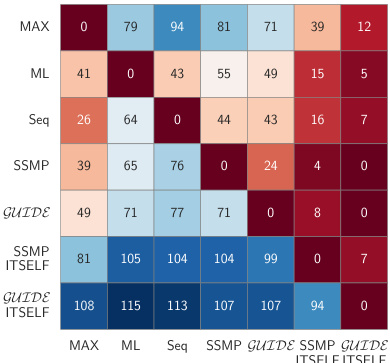
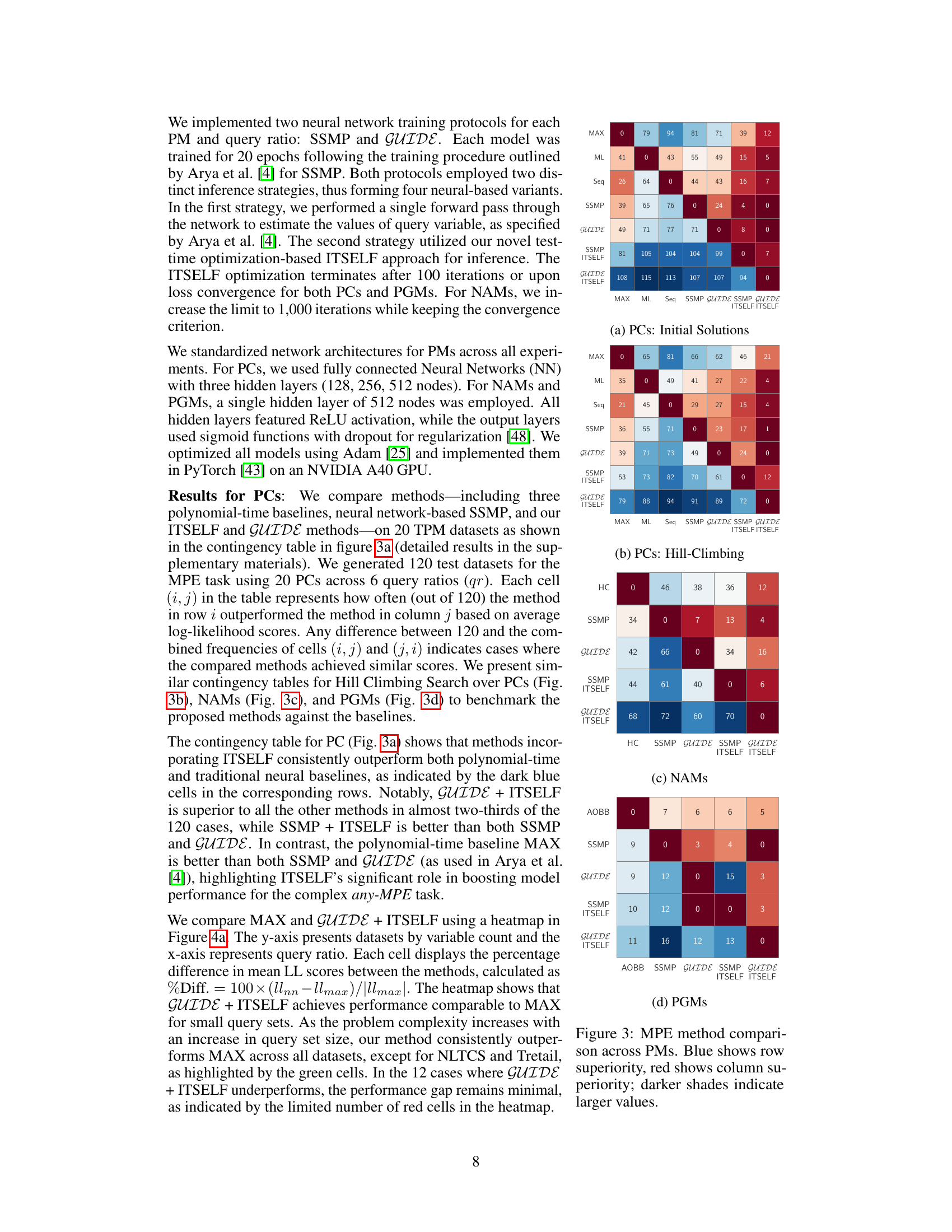
This contingency table summarizes the performance comparison between different MPE methods (MAX, ML, Seq, SSMP, GUIDE, SSMP+ITSELF, GUIDE+ITSELF) across various probabilistic models (PCs, NAMs, PGMs). Each cell (i, j) indicates how often method i outperformed method j in terms of average log-likelihood scores over 120 test datasets. Darker blue shades signify frequent wins for the row method, while darker red shades indicate more wins for the column method. The results visually demonstrate the effectiveness of the proposed ITSELF inference strategy, particularly when combined with the GUIDE training approach.
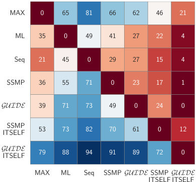
This figure presents contingency tables that compare the performance of different MPE (Most Probable Explanation) methods across various probabilistic models (PMs). The rows represent different methods, including polynomial-time baselines (MAX, ML, Seq) and the neural network-based methods proposed in the paper (SSMP, GUIDE, SSMP+ITSELF, GUIDE+ITSELF). The columns also represent different methods. Each cell (i, j) in a table shows how often (out of 120) method i outperformed method j based on average log-likelihood scores. A darker shade indicates a higher frequency of method i outperforming method j. The figure contains four sub-figures (a, b, c, d), each focusing on a specific type of probabilistic model: (a) Probabilistic Circuits (PCs), (b) PCs with Hill Climbing, (c) Neural Autoregressive Models (NAMs), and (d) Probabilistic Graphical Models (PGMs).
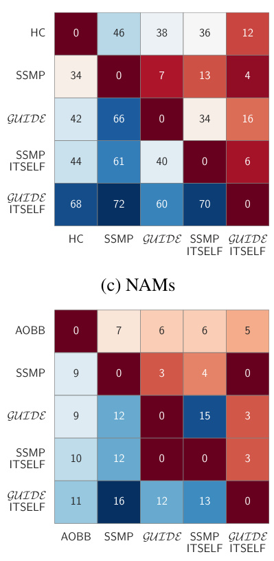
This figure presents a comparison of different methods for solving the Most Probable Explanation (MPE) task across various probabilistic models (PMs). It shows contingency tables visualizing the frequency with which each method outperforms others in terms of log-likelihood scores. The PMs include Probabilistic Circuits (PCs), Neural Autoregressive Models (NAMs), and Probabilistic Graphical Models (PGMs). The methods being compared are various baselines along with the proposed methods (SSMP, GUIDE, ITSELF) for solving the MPE problem. Darker blue shades indicate that a given method in a row frequently outperforms the method in the corresponding column, while darker red shades suggest the opposite.
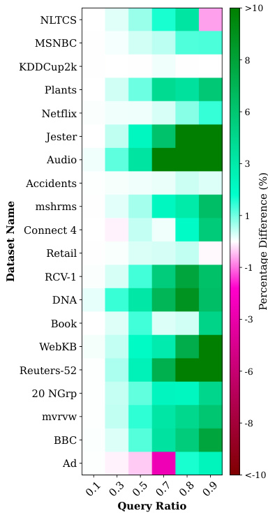
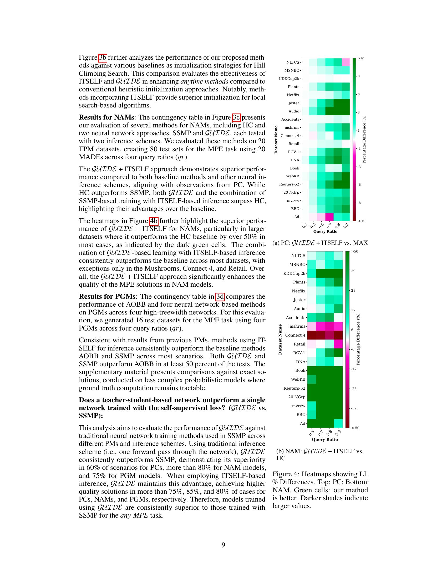
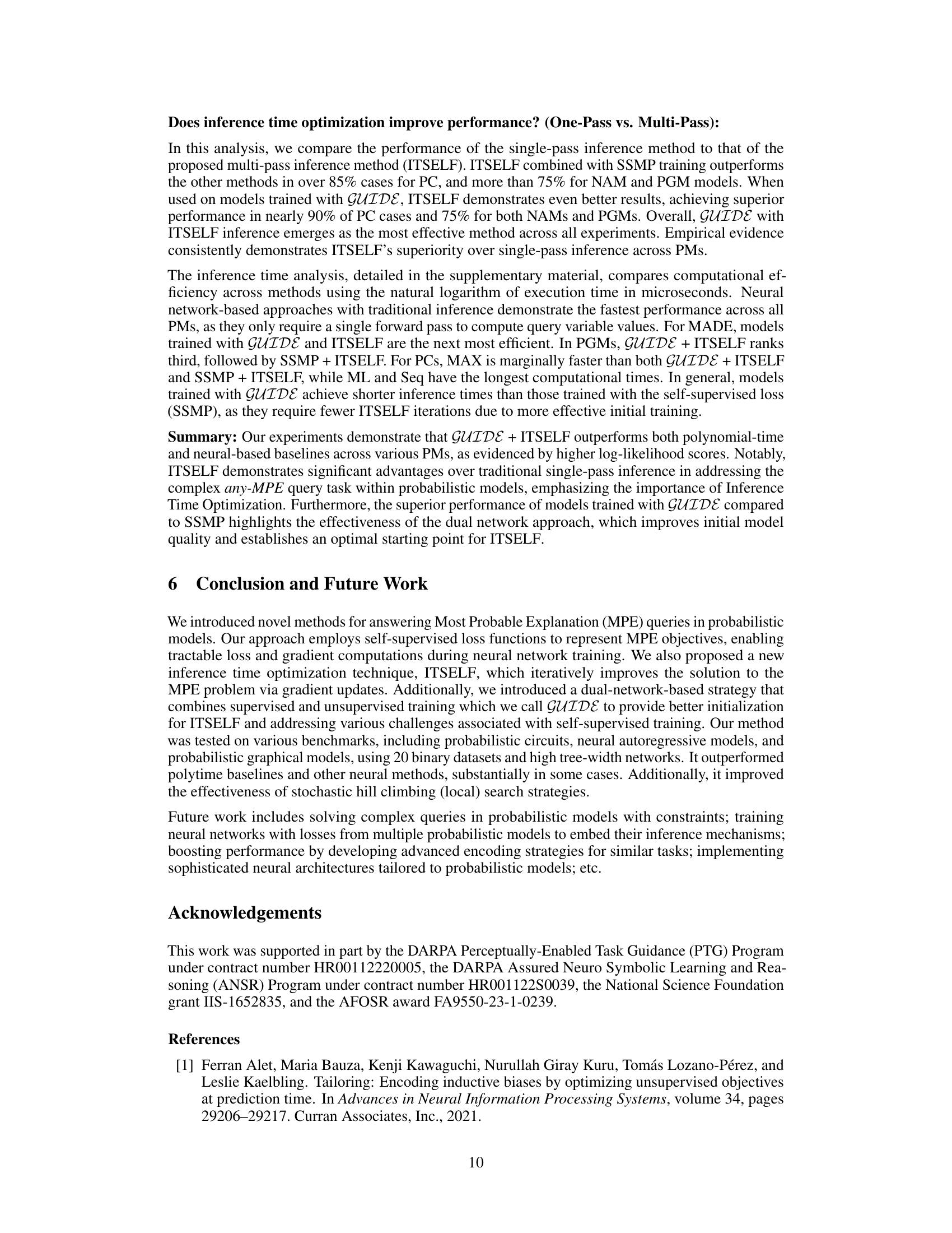
This figure presents two heatmaps visualizing the percentage difference in mean log-likelihood scores between the proposed GUIDE + ITSELF method and the MAX baseline across various datasets and query ratios. The top heatmap shows results for Probabilistic Circuits (PCs), while the bottom heatmap shows results for Neural Autoregressive Models (NAMs). Each cell in the heatmaps represents the percentage difference calculated as 100 * (ll_nn - ll_max) / |ll_max|, where ll_nn is the mean log-likelihood score of GUIDE + ITSELF, and ll_max is the mean log-likelihood score of the MAX baseline. Green cells indicate that GUIDE + ITSELF outperforms MAX. Darker shades of green represent larger performance gains.
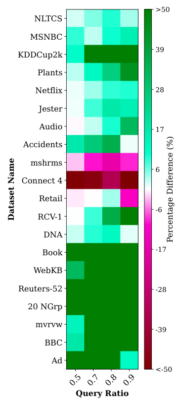
This figure presents two heatmaps visualizing the percentage difference in mean log-likelihood (LL) scores between the proposed GUIDE+ITSELF method and the MAX baseline for Probabilistic Circuits (PCs) and Neural Autoregressive Models (NAMs). The x-axis represents the query ratio, and the y-axis shows various datasets. Green cells indicate datasets where GUIDE+ITSELF outperforms MAX, while darker shades of green correspond to larger performance gains. The top heatmap displays results for PCs, and the bottom heatmap displays results for NAMs.
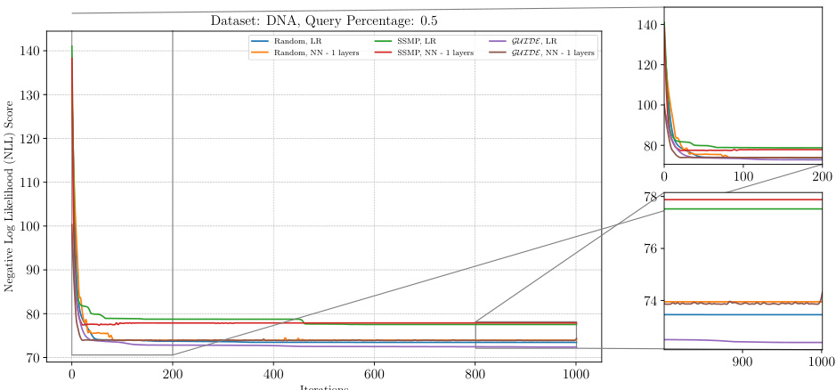
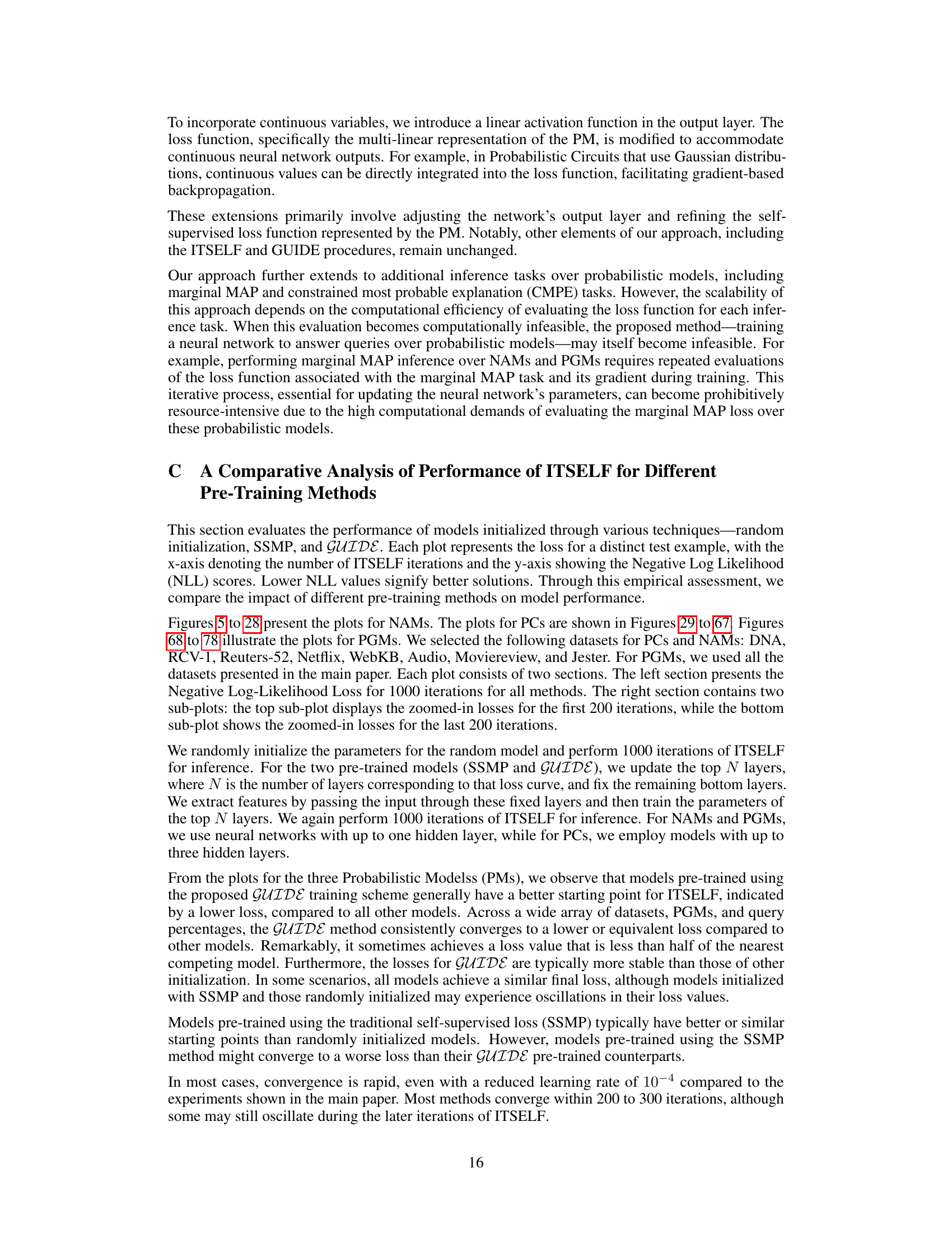
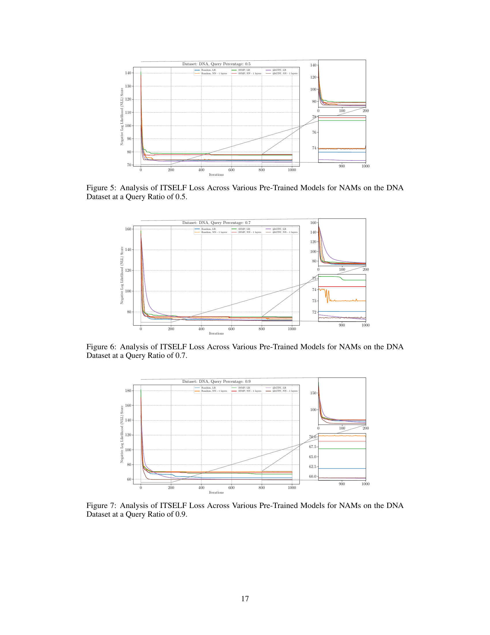
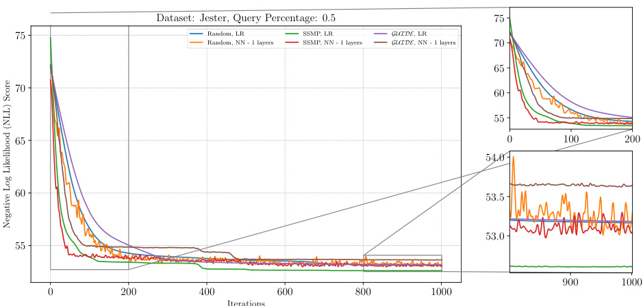
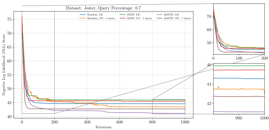
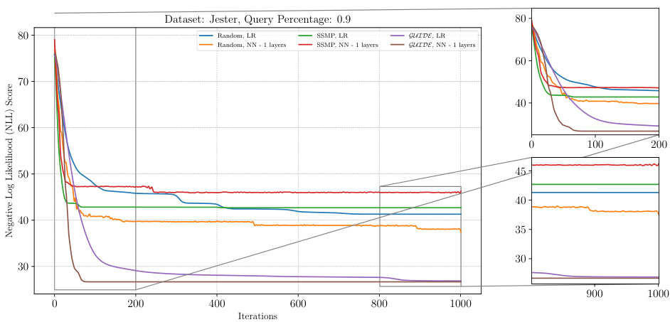
This figure shows the negative log-likelihood (NLL) loss across different iterations of the ITSELF algorithm for Neural Autoregressive Models (NAMs) on the DNA dataset with a query ratio of 0.5. Different lines represent different pre-trained models: Random (with and without 1 layer), SSMP (with and without 1 layer), and GUIDE (with and without 1 layer). The left panel displays the overall loss curve for all 1000 iterations. The right panel shows zoomed-in views of the first 200 iterations and the last 200 iterations, highlighting the convergence behavior of different models. The purpose is to demonstrate the impact of different pre-training methods on the performance of ITSELF in refining the MPE solution over time.
This figure analyzes the performance of ITSELF (Inference Time Self-Supervised Training) across various pre-trained models for Neural Autoregressive Models (NAMs) on the DNA dataset with a query ratio of 0.9. It shows how the negative log-likelihood loss changes over 1000 ITSELF iterations. Different lines represent different pre-training methods: Random (with and without one hidden layer), SSMP (supervised and self-supervised), and GUIDE (teacher-student). The subplots provide zoomed-in views of the loss curves during the initial and final 200 iterations for better understanding. The purpose is to demonstrate the effectiveness of different pre-training methods on the convergence behavior and final loss value of ITSELF.
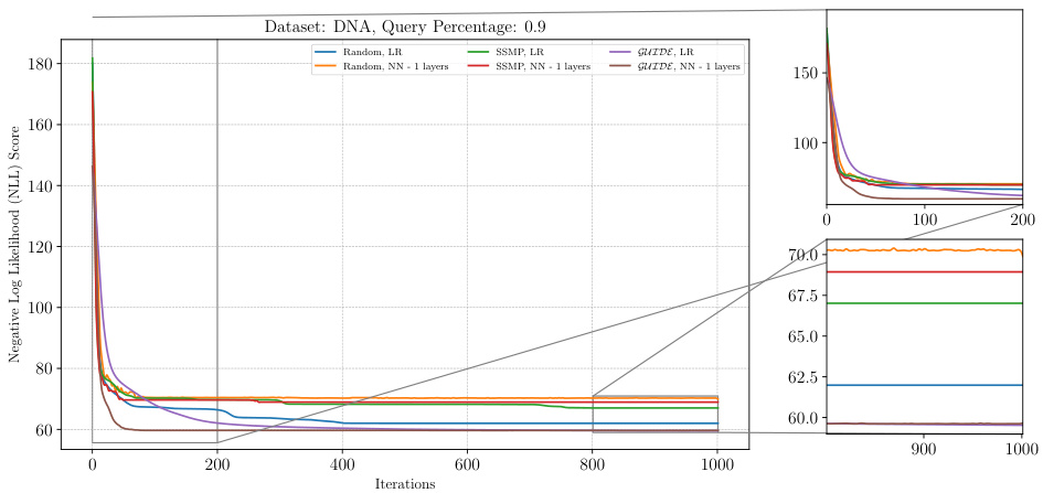
This figure visualizes the performance of the ITSELF algorithm across various pre-trained models (random, SSMP, and GUIDE) for Neural Autoregressive Models (NAMs) on the DNA dataset with a query ratio of 0.9. The main plot shows the negative log-likelihood loss over 1000 iterations of ITSELF. The zoomed-in plots on the right illustrate the convergence behavior in the initial and final 200 iterations. Different lines represent different model initializations and architectures (LR represents Logistic Regression). The goal is to demonstrate the effect of different pre-training methods on the convergence speed and final loss achieved by ITSELF.
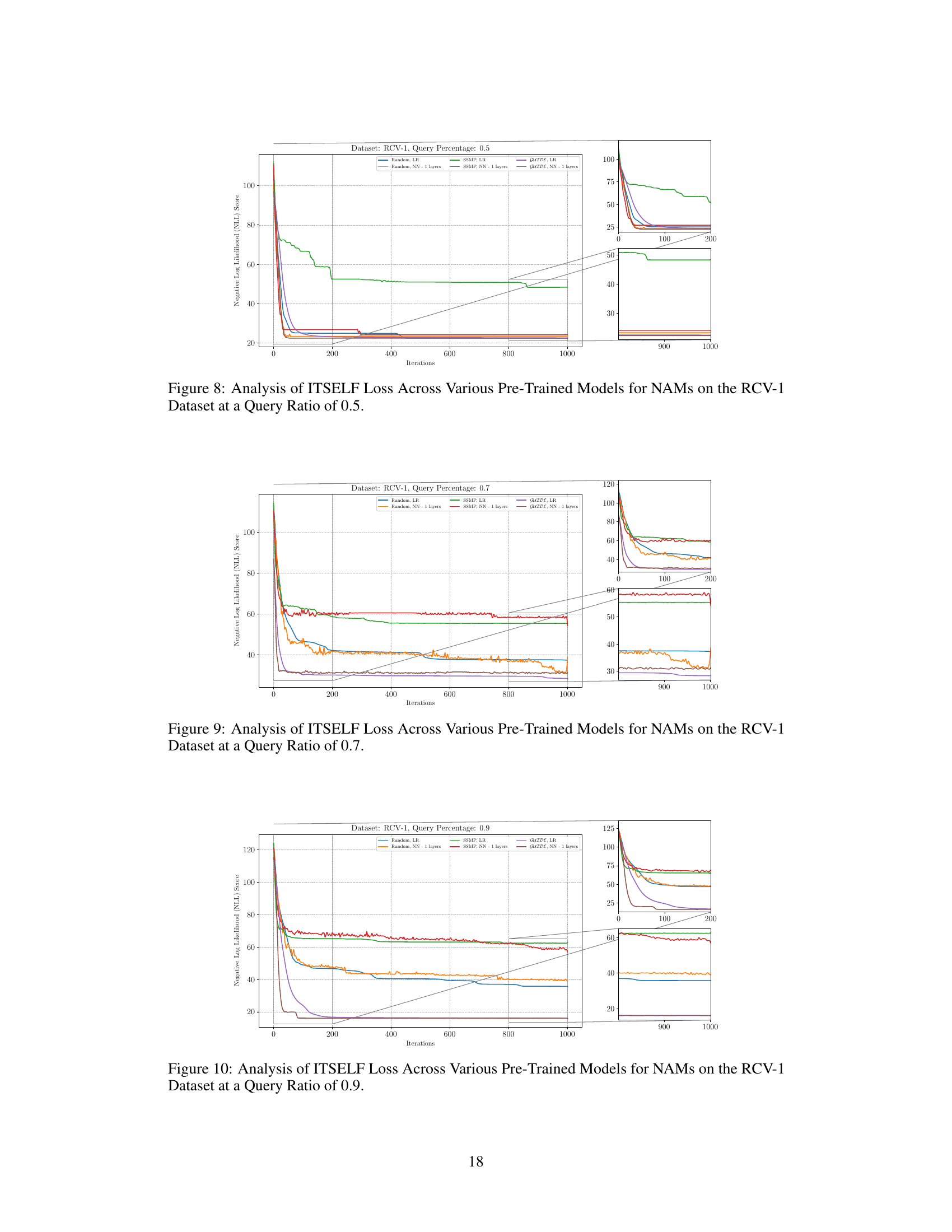
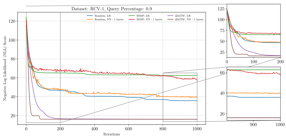
This figure displays the negative log-likelihood (NLL) loss values over 1000 iterations of the ITSELF algorithm for different pre-trained models applied to the RCV-1 dataset. The models used are trained with either supervised learning (GUIDE) or self-supervised learning (SSMP) and have 1 or 3 hidden layers. In addition to the models with pre-training, results for the randomly initialized models are also shown. The plot shows the significant impact of pre-training methods (GUIDE and SSMP) on improving the results of the algorithm’s convergence to a lower loss compared to a randomly initialized model.
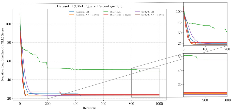
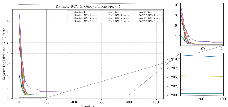
The figure shows the results of applying the ITSELF algorithm (Inference Time Self Supervised Training) on the RCV-1 dataset with a query ratio of 0.5. Different pre-trained models (Random, SSMP, GUIDE) were used as initializations for the network. The x-axis represents the number of iterations, while the y-axis shows the negative log-likelihood (NLL) loss. The plot visually compares the convergence speed and final NLL loss achieved by each model. The zoomed-in plots emphasize the behavior in the early and late stages of training.
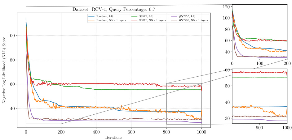
This figure presents a detailed analysis of the ITSELF (Inference Time Self-Supervised Training) loss across various pre-trained models for Neural Autoregressive Models (NAMs) on the RCV-1 dataset. The x-axis represents the number of ITSELF iterations, and the y-axis shows the negative log-likelihood (NLL) score. Different lines represent different pre-training methods (Random, SSMP, GUIDE) combined with different numbers of neural network layers (LR indicating Logistic Regression). The main plot shows the overall loss during ITSELF iterations, while the inset shows the zoomed-in loss at both the beginning and the end of iterations. This visualization aids in comparing the convergence behaviors and the final loss values achieved by different pre-training methods.
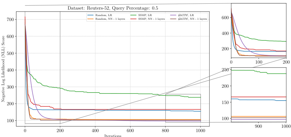
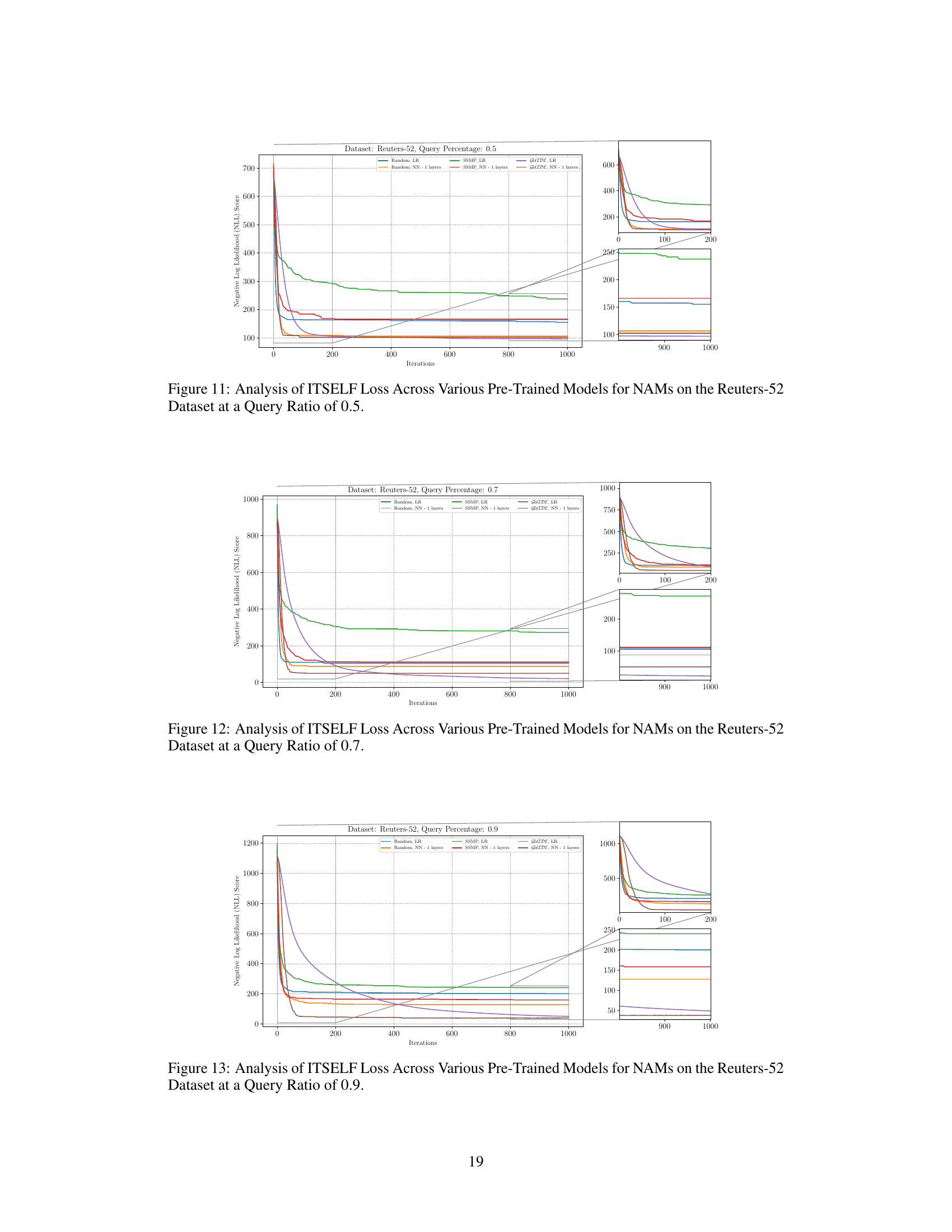
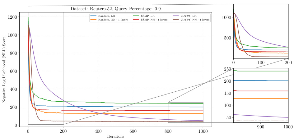
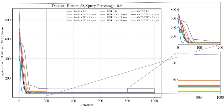
This figure illustrates the performance of the ITSELF algorithm across different pre-trained models for Neural Autoregressive Models (NAMs) on the Reuters-52 dataset with a query ratio of 0.9. The x-axis represents the number of ITSELF iterations, and the y-axis shows the negative log-likelihood (NLL) score. Lower NLL scores indicate better model performance. The plot shows the loss curves for models initialized randomly (with and without additional layers) and models pre-trained using SSMP and GUIDE (again with and without additional layers). The zoomed-in plots at the lower right show the loss convergence behaviour in the early and later stages of training.
The figure shows the negative log-likelihood loss values over 1000 iterations of the ITSELF algorithm for PCs on the Reuters-52 dataset with a query ratio of 0.9. Multiple lines represent different model initializations: random initialization with logistic regression (Random, LR), random initialization with varying numbers of neural network hidden layers (Random, NN-1, -2, -3 layers), self-supervised training with logistic regression (SSMP, LR), self-supervised training with varying numbers of neural network hidden layers (SSMP, NN-1, -2, -3 layers), guided iterative dual learning with logistic regression (GUIDE, LR), and guided iterative dual learning with varying numbers of neural network hidden layers (GUIDE, NN-1, -2, -3 layers). The plot helps visualize how different initialization methods affect the convergence speed and final loss achieved by ITSELF.
This figure presents a detailed analysis of the ITSELF (Inference Time Self-Supervised Training) loss across various pre-trained models for Probabilistic Circuits (PCs) on the Reuters-52 dataset with a query ratio of 0.9. The plot displays the negative log-likelihood (NLL) loss over 1000 iterations of ITSELF. Multiple lines represent different model initializations: Random (with and without layer-wise training), SSMP (Self-Supervised MPE in PCs), and GUIDE (Guided Iterative Dual Learning with Self-supervised Teacher). The subplots provide zoomed-in views of the initial and final 200 iterations to highlight the convergence behavior of each method.
This figure shows the analysis of the ITSELF loss across different pre-trained models for Neural Autoregressive Models (NAMs) on the DNA dataset with a query ratio of 0.5. The x-axis represents the number of ITSELF iterations, and the y-axis represents the negative log-likelihood (NLL) score. Lower NLL scores indicate better performance. The plot shows the performance of models initialized with random parameters, SSMP, and GUIDE. Each model is tested with two different neural network architectures, one with a single hidden layer and another with a single linear layer for comparison.

The figure shows the negative log-likelihood loss for different neural network models trained with various initialization methods (random, SSMP, GUIDE) on the DNA dataset with a query ratio of 0.9. Each line represents a different initialization method and network architecture (LR: Logistic Regression, NN-1 layers: Neural Network with one hidden layer). The x-axis shows the number of ITSELF iterations, while the y-axis shows the loss. The zoomed-in sections highlight the initial and final phases of training to better visualize the convergence behavior of different models. The plot demonstrates the efficacy and scalability of the approach using self-supervised loss.
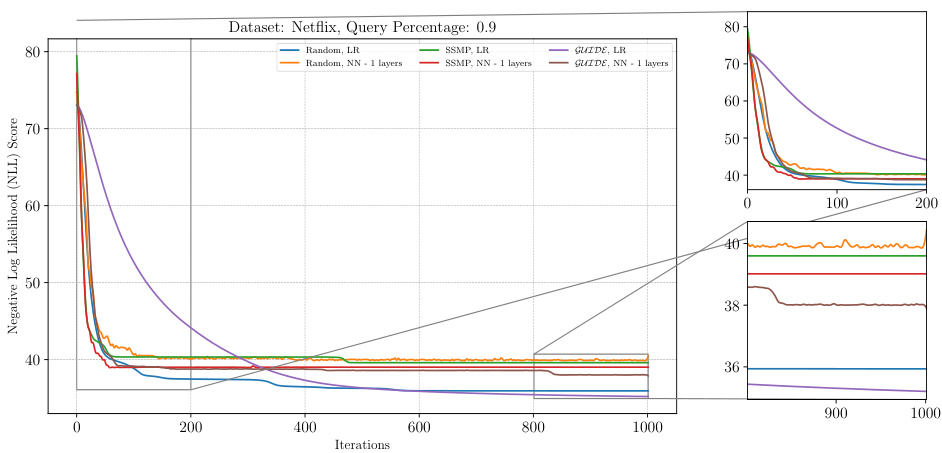
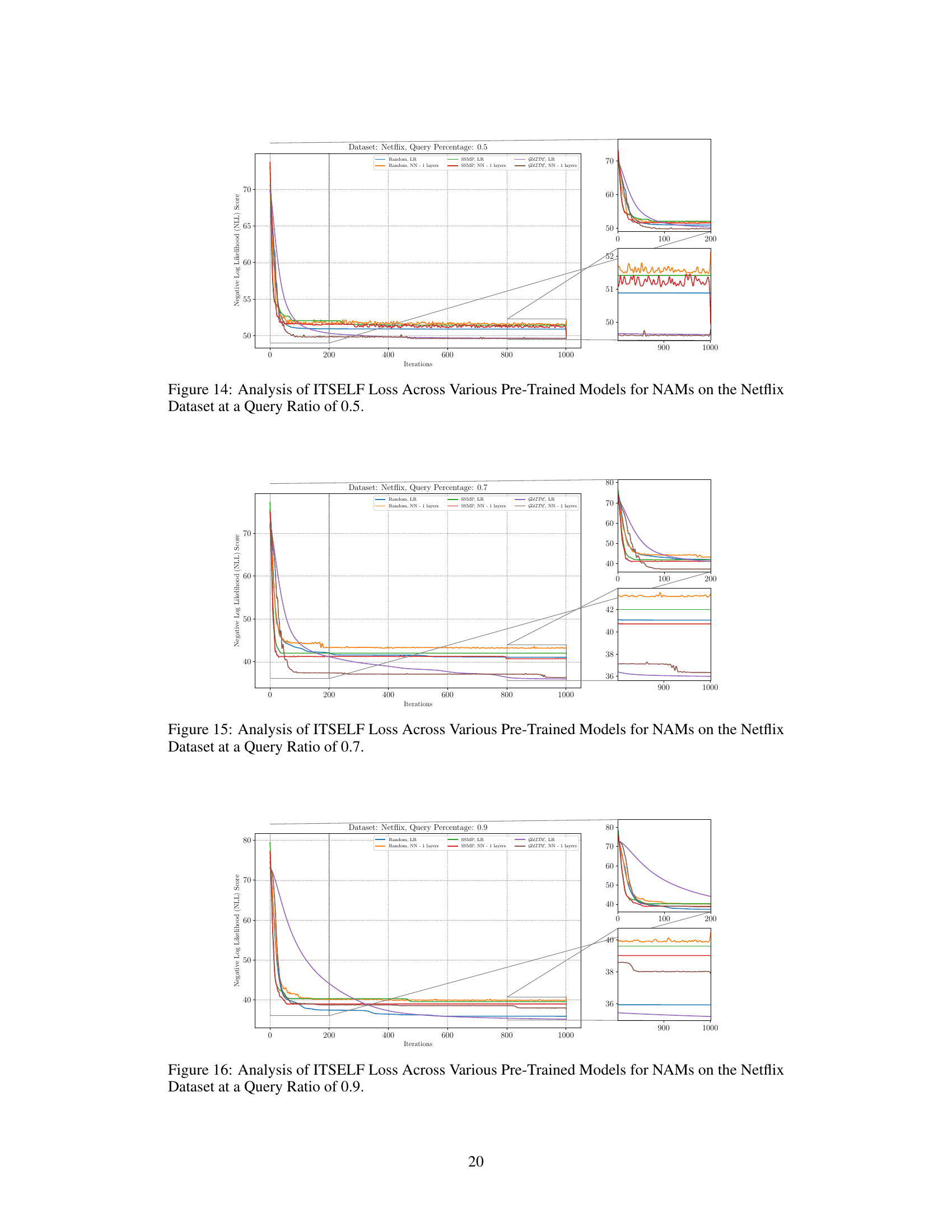
The figure shows the analysis of ITSELF loss across various pre-trained models for PCs on the Netflix dataset at a query ratio of 0.9. The x-axis represents the number of iterations, while the y-axis represents the negative log-likelihood (NLL) score. Different colored lines represent the different models trained using various methods such as random initialization, SSMP, and GUIDE, each with and without using 1 layer neural networks. The zoomed in plots for iterations 0-200 and 900-1000 are also shown. The graph helps in comparing performance of different models and training methods based on the convergence speed and loss values.
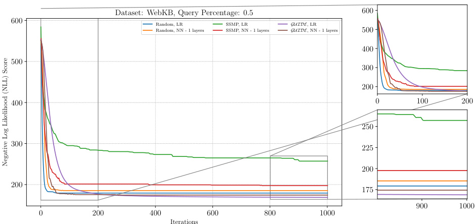
The figure shows the loss curves obtained by applying ITSELF (Inference Time Self-Supervised Training) with different pre-trained models for PCs on the WebKB dataset with a query ratio of 0.1. The pre-trained models used are Random, SSMP, and GUIDE, each with and without an additional hidden layer. The plot shows the negative log-likelihood loss over 1000 iterations. In the zoomed in plots, the loss curves are very close for iterations 900-1000, and GUIDE, LR achieves better performance compared to others.
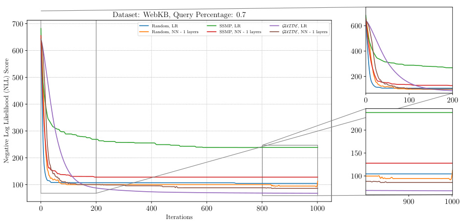
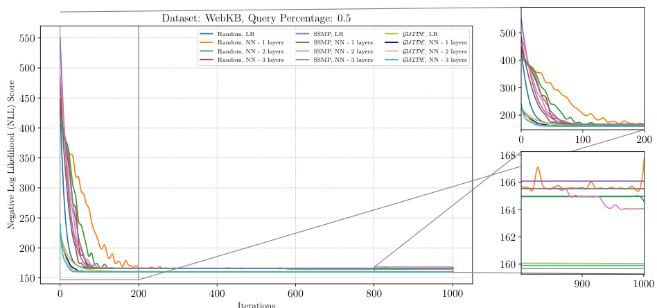
This figure analyzes the performance of the ITSELF algorithm across different pre-trained models (Random, SSMP, and GUIDE) for Neural Autoregressive Models (NAMs) on the WebKB dataset with a query ratio of 0.5. The x-axis represents the number of ITSELF iterations, and the y-axis shows the negative log-likelihood (NLL) score. Lower NLL scores indicate better model performance. The figure shows that models pre-trained using GUIDE generally converge to a lower loss compared to other models, demonstrating its effectiveness in improving the initialization point for ITSELF. The zoomed-in plots for both early and later iterations showcase this difference in performance.
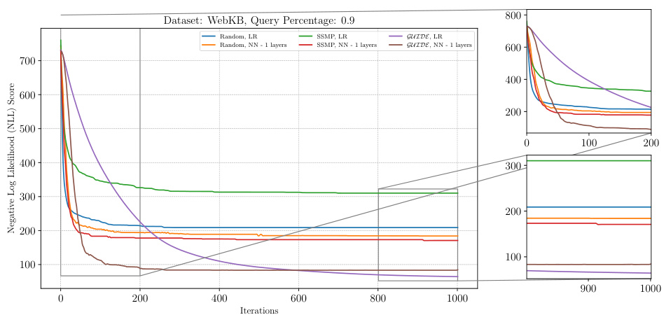
The figure shows the negative log-likelihood loss values over 1000 ITSELF iterations for PCs on the WebKB dataset with a query ratio of 0.5. Multiple lines represent different model pre-training methods (Random, SSMP, GUIDE) and whether or not a single or multiple hidden layers were used. The plot allows for a comparison of the convergence speed and final loss values across various initialization strategies.
This figure displays the negative log-likelihood loss (NLL) over 1000 iterations of ITSELF for different pre-trained models on the DNA dataset. The query ratio is 0.5. The models were pre-trained using random initialization, SSMP, and GUIDE, each with different numbers of layers. The subplots provide zoomed-in views on the first 200 and last 200 iterations. The results showcase the impact of different pre-training methods on the convergence rate and final loss achieved during the ITSELF optimization process.
The figure shows the loss curves of ITSELF across various pre-trained models for Neural Autoregressive Models (NAMs) on the DNA dataset at a query ratio of 0.9. It compares different initialization methods (Random, SSMP, GUIDE) with and without an additional layer in the NN architecture. The plot illustrates the negative log likelihood (NLL) loss over 1000 iterations of ITSELF. The zoomed-in subplots highlight the initial and final 200 iterations of the loss convergence. This allows a detailed analysis of convergence behavior for each initialization strategy and helps understand the effect of the added NN layer on the optimization process.
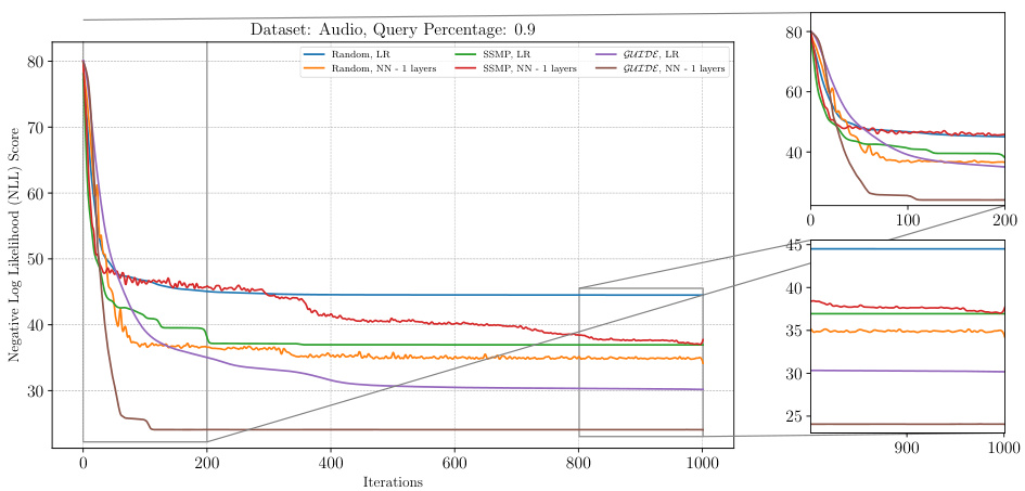
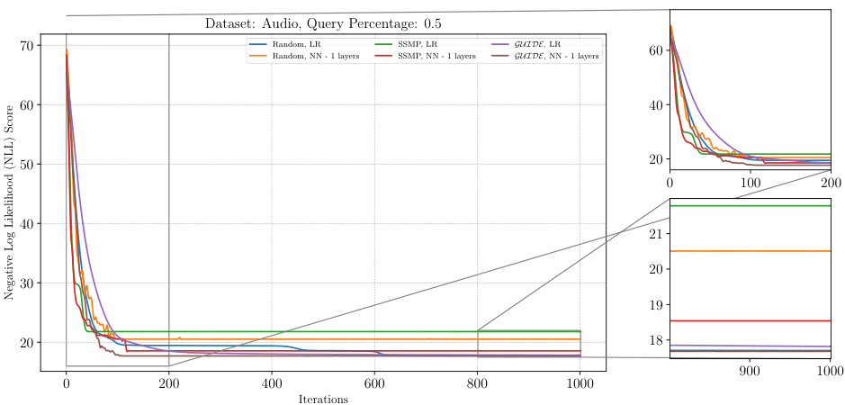
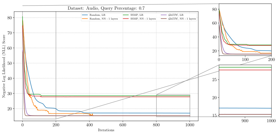
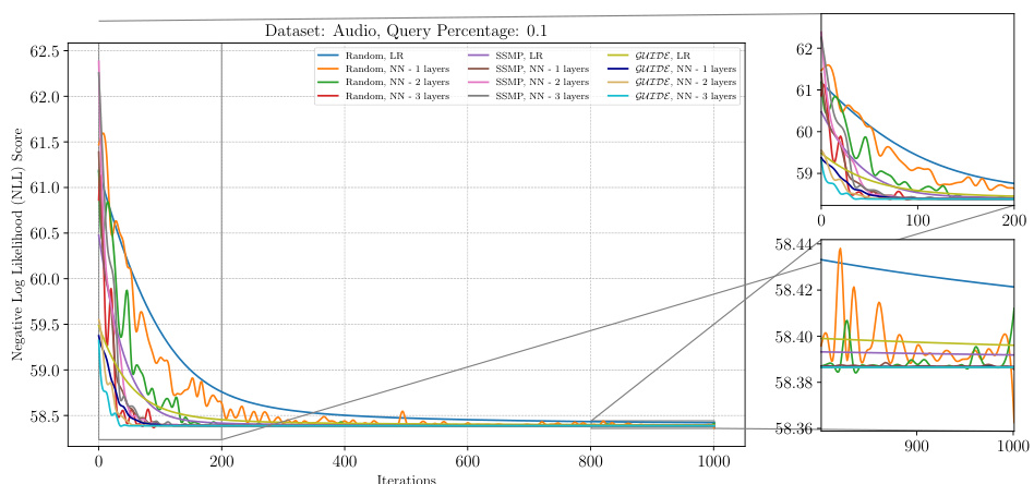
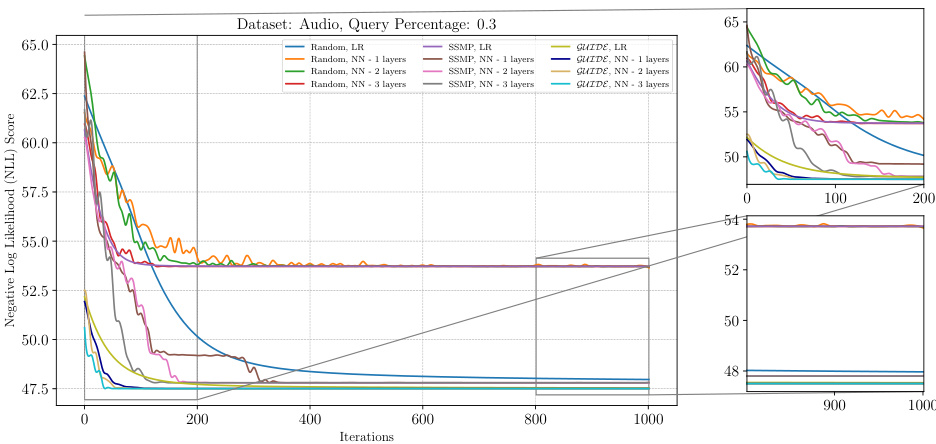
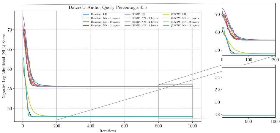
The figure shows the results of applying the ITSELF algorithm to various pre-trained models for Probabilistic Circuits (PCs) on the Audio dataset. The x-axis represents the number of iterations of the ITSELF algorithm, and the y-axis represents the negative log-likelihood (NLL) score, a measure of model performance. Different lines represent different pre-trained models, each with various numbers of hidden layers and using different training methods (Random, SSMP, GUIDE). The plot helps visualize the convergence behavior of each model during the inference-time optimization process. The goal is to observe how quickly and effectively each model converges to a low NLL score (indicating improved MPE solution accuracy). The zoomed-in subplots offer greater detail during the initial and final phases of the optimization process.
This figure analyzes the performance of the ITSELF algorithm (Inference Time Self-Supervised Training) for PCs on the DNA dataset with a query ratio of 0.5. It compares the loss across different pre-trained models: Random (with and without additional layers), SSMP (Self-Supervised MPE in PCs, with and without additional layers), and GUIDE (Guided Iterative Dual Learning with Self-supervised Teacher, with and without additional layers). The x-axis represents the number of ITSELF iterations, and the y-axis represents the negative log-likelihood (NLL) score. Lower NLL scores indicate better model performance. The figure shows the loss curves for each model, allowing for a comparison of their convergence behavior and final performance.
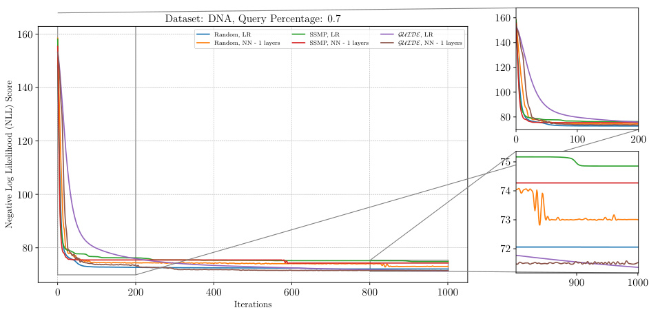
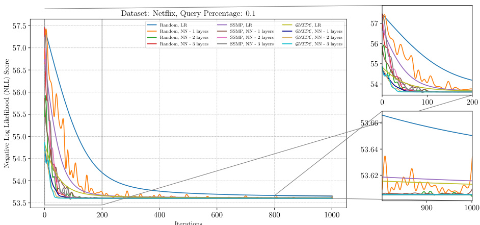
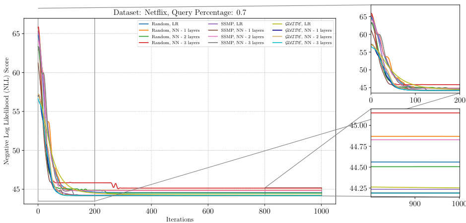
The figure shows the negative log-likelihood loss for different pre-trained models (random, SSMP, and GUIDE) on the Netflix dataset with a query ratio of 0.7. Each line represents a different model architecture and training method. The x-axis represents the number of ITSELF iterations, and the y-axis represents the negative log-likelihood score. The plot includes zoomed-in views of the loss for both early and late iterations, illustrating the convergence behavior of different initialization strategies. Lower NLL scores are better.
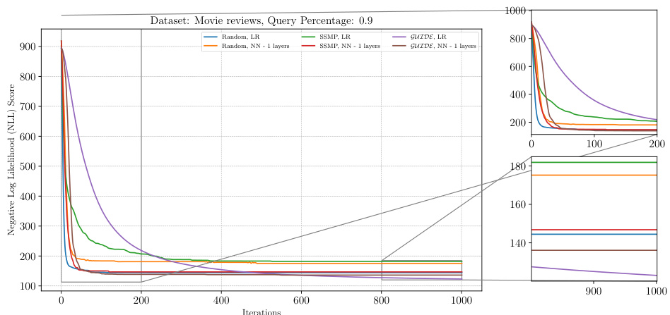
The figure shows the Negative Log Likelihood (NLL) scores over 1000 iterations of the ITSELF algorithm for PCs on the Netflix dataset with a query ratio of 0.9. Different lines represent different model initialization strategies, including random initialization with and without one hidden layer, SSMP (Self-Supervised learning based MMAP solver for PCs) pre-training with and without one hidden layer, and GUIDE (GUided Iterative Dual LEarning with Self-supervised Teacher) pre-training with and without one hidden layer. The plot allows for a comparison of the convergence behavior of different model training methods, and demonstrates how the various initialization methods affect the starting point and speed of convergence of the ITSELF algorithm.
The figure shows the negative log-likelihood loss values over 1000 iterations of the ITSELF algorithm for different pre-trained models (random, SSMP, and GUIDE) on the Netflix dataset with a query ratio of 0.9. The loss values represent the quality of MPE solutions obtained at each iteration using a neural network with one hidden layer. The plot includes zoomed-in sections for the initial and final 200 iterations to show details of the loss convergence behavior. The results highlight how the choice of pre-training affects the loss convergence during the inference optimization process.
The figure illustrates the convergence behavior of the ITSELF algorithm across different pre-trained models (Random, SSMP, and GUIDE) for Neural Autoregressive Models (NAMs) on the Netflix dataset with a query ratio of 0.7. It shows how the negative log-likelihood loss decreases over 1000 iterations. The different lines represent different model initializations, demonstrating the impact of pre-training on the efficiency and effectiveness of ITSELF.
The figure shows the result of applying the ITSELF algorithm for different pre-trained models on the Netflix dataset with a query ratio of 0.9. The plot illustrates the negative log-likelihood loss across 1000 iterations of the ITSELF optimization. Different lines represent different model initializations: random with linear regression, random with a neural network of 1 layer, SSMP pre-trained with linear regression, SSMP pre-trained with a neural network of 1 layer, GUIDE pre-trained with linear regression and GUIDE pre-trained with a neural network of 1 layer. The plot shows how the loss converges for each initialization method, with a focus on the difference between self-supervised (SSMP) and teacher-student (GUIDE) pre-training methods.

The figure displays the analysis of ITSELF loss across various pre-trained models for Probabilistic Circuits (PCs) on the DNA dataset at a query ratio of 0.1. It shows the negative log-likelihood (NLL) score plotted against the number of iterations. Multiple lines represent different model initializations (Random, SSMP, GUIDE) and network architectures (LR, 1-3 layers). The plot illustrates how the loss converges over iterations for each model, demonstrating the effectiveness of the ITSELF optimization technique for different model initializations and architectures. A zoomed-in portion provides a clearer view of the loss convergence in the later iterations.
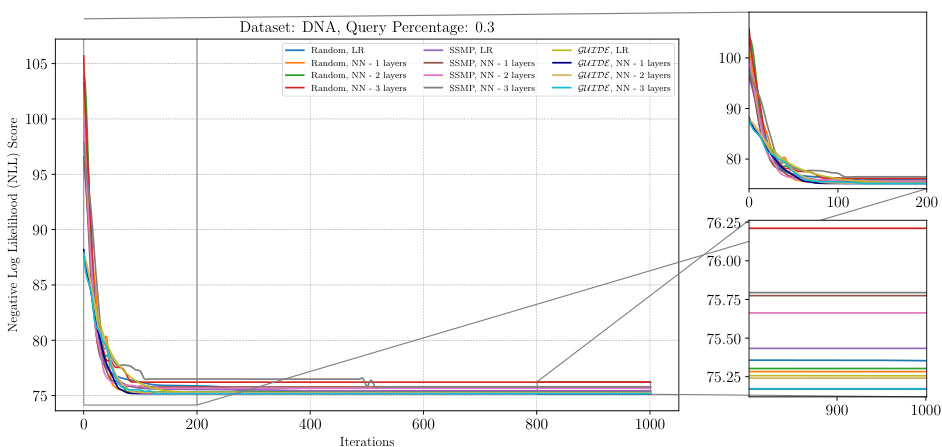
The figure shows the analysis of ITSELF loss across various pre-trained models for PCs on the DNA dataset at a query ratio of 0.3. It displays the negative log-likelihood (NLL) score on the y-axis versus the number of iterations on the x-axis. Multiple lines represent different pre-training methods (Random, SSMP, GUIDE), each with different numbers of layers in the neural network architecture. The plot illustrates how each model’s loss decreases over the iterations of ITSELF (Inference Time Self Supervised Training). The zoomed in plots in the right panel show the detailed performance in early and late stages of the ITSELF iterations.
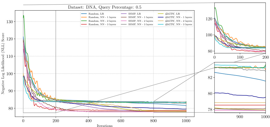
This figure displays the negative log-likelihood loss values over 1000 iterations of ITSELF for different pre-trained models on the DNA dataset with a query ratio of 0.5. The models are categorized by pre-training method (Random, SSMP, GUIDE) and number of layers in the neural network architecture. The plot shows how the loss changes with each iteration of the ITSELF algorithm, indicating the convergence behavior of each model. It demonstrates the impact of pre-training strategies (Random, Self-Supervised, and Teacher-Student) and network architectures on the optimization process of ITSELF.
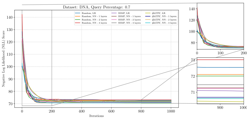
The figure shows the performance of ITSELF (Inference Time Self-Supervised Training) across various pre-trained models for Probabilistic Circuits (PCs) on the DNA dataset with a query ratio of 0.5. The x-axis represents the number of ITSELF iterations, and the y-axis represents the negative log-likelihood (NLL) score. Lower NLL scores indicate better performance. The plot compares different initialization methods: random initialization with and without different numbers of hidden layers in the neural network, as well as models pre-trained using SSMP (Self-Supervised MPE for PCs) and GUIDE (Guided Iterative Dual Learning with Self-supervised Teacher). The plot visually demonstrates how the different initialization methods impact the convergence speed and final NLL score achieved by ITSELF during inference.
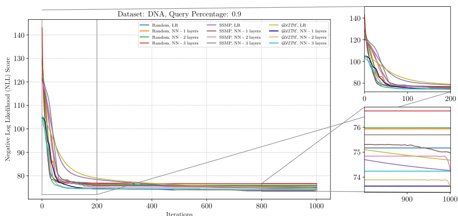
This figure shows the result of applying the ITSELF algorithm to various pre-trained models for Probabilistic Circuits (PCs) on the DNA dataset with a query ratio of 0.9. The x-axis represents the number of iterations of the ITSELF algorithm, and the y-axis shows the negative log-likelihood (NLL) score, a measure of model accuracy. Different lines represent different pre-training methods (Random, SSMP, GUIDE) and different network architectures (LR, NN with 1-3 layers). The plots showcase how different initialization strategies impact convergence speed and final loss values.
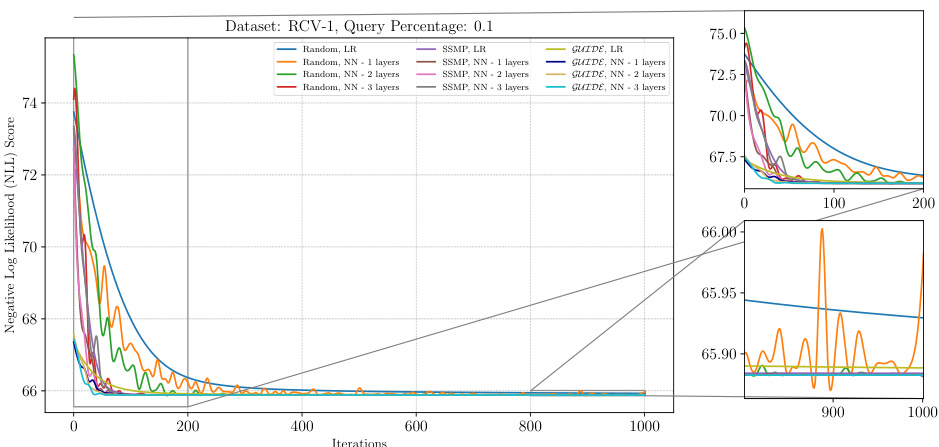
The figure shows the negative log-likelihood loss values over 1000 iterations of the ITSELF algorithm for various pre-trained models on the RCV-1 dataset with a query ratio of 0.1. The models include those initialized randomly (with and without using neural networks with varying numbers of layers), those pre-trained using the SSMP method, and those pre-trained using the GUIDE method. The plot allows one to visualize and compare the convergence behavior of different initialization strategies in terms of achieving lower loss values (better performance) during the inference process. The zoomed-in plots highlight the convergence behavior during the initial (0-200 iterations) and final (900-1000 iterations) stages of the ITSELF inference process.
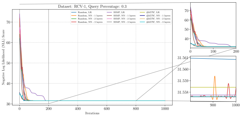
The figure displays the negative log-likelihood loss across 1000 ITSELF iterations for different pre-trained models on the RCV-1 dataset with a query ratio of 0.3. Each line represents a different model, showing the convergence of the loss function over time for various initialization strategies (Random, SSMP, GUIDE). The plots are split into three parts, the main plot shows the entire training process; while the smaller plots zoom into the start and end of the training, respectively, illustrating the behavior of the models at various stages of learning.
This figure shows the negative log-likelihood loss across iterations of ITSELF for various pre-trained models (Random, SSMP, GUIDE) applied to NAMs on the DNA dataset with a query ratio of 0.5. The plot demonstrates how the loss changes as the model iteratively refines the MPE solution using inference-time self-supervised training (ITSELF). The different lines represent the performance of different pre-training strategies and network architectures (using linear regression or neural networks with varying numbers of layers). The zoomed-in sub-plots offer a detailed view of the initial and final iterations, highlighting the convergence behavior of each approach.
This figure shows the results of applying the Inference Time Self Supervised Training (ITSELF) algorithm to different pre-trained models for Probabilistic Circuits (PCs) on the DNA dataset. The x-axis represents the number of ITSELF iterations, and the y-axis shows the negative log-likelihood loss. Different colored lines represent different pre-training methods (random initialization, SSMP, and GUIDE) and different network architectures (varying number of layers). The smaller zoomed plots on the right show the initial and later stages of the loss curves, highlighting convergence trends. This helps illustrate how different pre-training methods impact the speed and efficiency of achieving low loss in the ITSELF optimization.
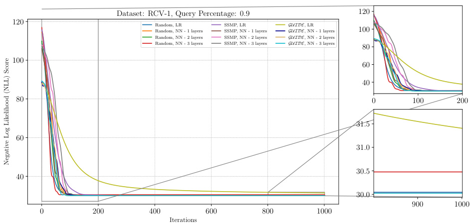
The figure shows the analysis of ITSELF loss across various pre-trained models for PCs on the DNA dataset at a query ratio of 0.9. The plot shows how the negative log-likelihood (NLL) loss changes over 1000 ITSELF iterations. The different lines represent different model training methods, such as using random initialization, SSMP (Self-Supervised MPE solver for PCs), and GUIDE (Guided Iterative Dual LEarning with Self-supervised Teacher). The subplots zoom into the first 200 and last 200 iterations to show details of convergence behavior. The plot provides a visual comparison of different training methods’ impact on the MPE task performance, specifically focusing on loss convergence within the ITSELF iterative optimization.
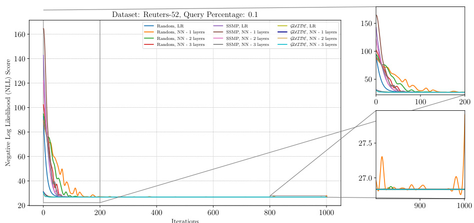
This figure presents a detailed analysis of the ITSELF (Inference Time Self-Supervised Training) loss across various pre-trained models for Probabilistic Circuits (PCs) on the Reuters-52 dataset at a query ratio of 0.9. The plot shows the negative log-likelihood loss (NLL) over 1000 iterations for different model initializations: random initialization with and without different numbers of hidden layers (1,2,3), SSMP (Self-Supervised MPE task) pre-training with different numbers of hidden layers, and GUIDE (Guided Iterative Dual Learning) pre-training with different numbers of hidden layers. The zoomed-in insets highlight the behavior of the models in the early and later iterations of the training process. This helps in understanding the convergence speed and stability of different methods under various training initializations.
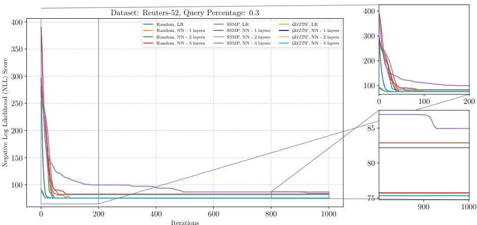
This figure displays the negative log-likelihood loss values for different model initialization methods across 1000 ITSELF iterations. The x-axis represents the number of iterations, and the y-axis shows the negative log-likelihood loss. The plot shows that the models pre-trained with the proposed GUIDE method tend to converge faster and to lower loss values compared to those initialized randomly or using the SSMP approach. The zoomed-in insets highlight the initial iterations and final convergence behavior for each training method.
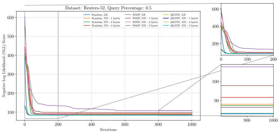
The figure shows the Negative Log Likelihood (NLL) scores over 1000 iterations of ITSELF for different pre-trained models on the Reuters-52 dataset with a query ratio of 0.9. The models include those with random initialization, pre-trained using SSMP (self-supervised learning), and pre-trained using GUIDE (a teacher-student approach). Different numbers of hidden layers (1, 2, and 3) are also shown for the neural network models. The plot illustrates how the loss converges over time for each model, providing insight into their training and optimization effectiveness.
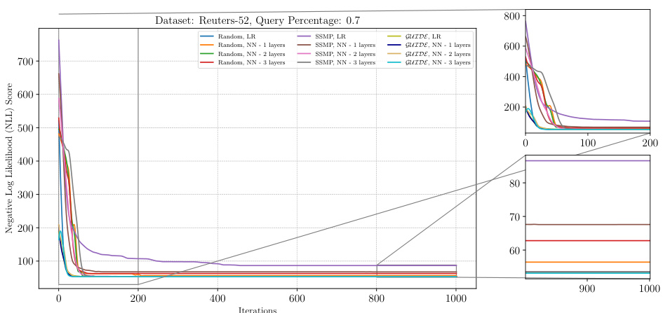
The figure visualizes the performance of the ITSELF algorithm across different pre-trained models for PCs on the Reuters-52 dataset with a query ratio of 0.9. It shows how the negative log-likelihood loss changes over 1000 iterations of ITSELF, comparing the performance of models initialized randomly, with SSMP (Self-Supervised MPE), and with GUIDE (Guided Iterative Dual Learning). Different line colors represent models trained with varying numbers of layers (1-3) within the neural network architecture.
This figure shows the negative log-likelihood loss for different PC models across 1000 iterations of ITSELF optimization. The models used include those initialized with various training methods: Random, SSMP, and GUIDE, and each with different numbers of hidden layers (1, 2, or 3). The plot shows the convergence behavior of the models under ITSELF, illustrating how different initialization strategies affect the optimization process and final loss. The x-axis represents the number of iterations, and the y-axis represents the negative log-likelihood loss. The smaller losses correspond to better solutions.
This figure displays the negative log-likelihood loss over 1000 iterations of ITSELF for NAMs on the DNA dataset with a query ratio of 0.5. Multiple lines represent different model initializations: random initialization with and without a single or multiple hidden layers; SSMP-trained models (using Self-Supervised learning) with and without multiple layers; GUIDE-trained models (using both Self-Supervised and supervised learning) with and without multiple layers. The plot shows how the loss value changes during the iterative ITSELF optimization process for each initialization method, providing insight into their convergence behavior and the effectiveness of different pre-training strategies.
This figure shows the negative log-likelihood (NLL) loss over 1000 iterations of ITSELF for different pre-trained models (random, SSMP, GUIDE) on the DNA dataset with a query ratio of 0.5. The plot includes subplots showing the first 200 and last 200 iterations for a more detailed view. The various lines represent different model types, including those trained with one, two, or three hidden layers, as well as those using learning rate reduction.
The figure shows the results of the Inference Time Self Supervised Training (ITSELF) algorithm across various pre-trained models on the DNA dataset for Neural Autoregressive Models (NAMs) with a query ratio of 0.5. The x-axis represents the number of iterations and the y-axis represents the negative log-likelihood (NLL) score. The plot shows the training curves of six different models: three models were initialized randomly and trained with the self-supervised loss function; and three others were trained with supervised learning (GUIDE) before performing the self-supervised optimization. For both training methods, three different neural network architectures were considered: one-layer, two-layer, and three-layer models. The results demonstrate the effectiveness of the GUIDE pre-training method. The models pre-trained with GUIDE tend to have lower NLL scores than randomly initialized models, and converge faster to the optimal solution.
The figure shows the result of applying the ITSELF algorithm (Inference Time Self Supervised Training) to various pre-trained models for Neural Autoregressive Models (NAMs) on the Reuters-52 dataset. The x-axis represents the number of ITSELF iterations, and the y-axis shows the negative log-likelihood (NLL) score. Lower NLL scores indicate better solutions. The different lines represent different initialization methods (random, SSMP, and GUIDE) and different NN architectures. The plot illustrates the convergence of the ITSELF algorithm towards near-optimal MPE solutions from various starting points. The inset plots provide a zoomed-in view of the early and late iterations.
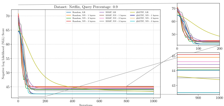
This figure displays the negative log-likelihood (NLL) scores over 1000 ITSELF iterations for various pre-trained models on the Netflix dataset with a query ratio of 0.9. Different lines represent different model training methods (random initialization, SSMP, and GUIDE) with varying numbers of hidden layers. The zoomed-in plots on the right show details of the loss curves for the initial 200 and the final 200 iterations.
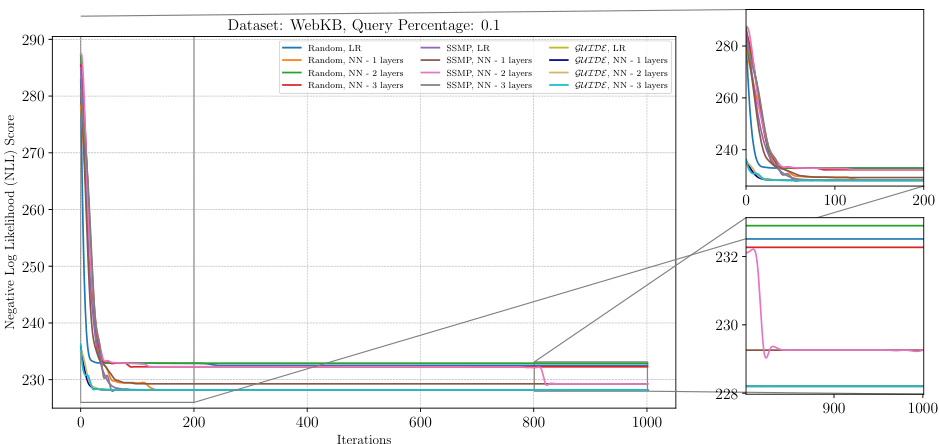
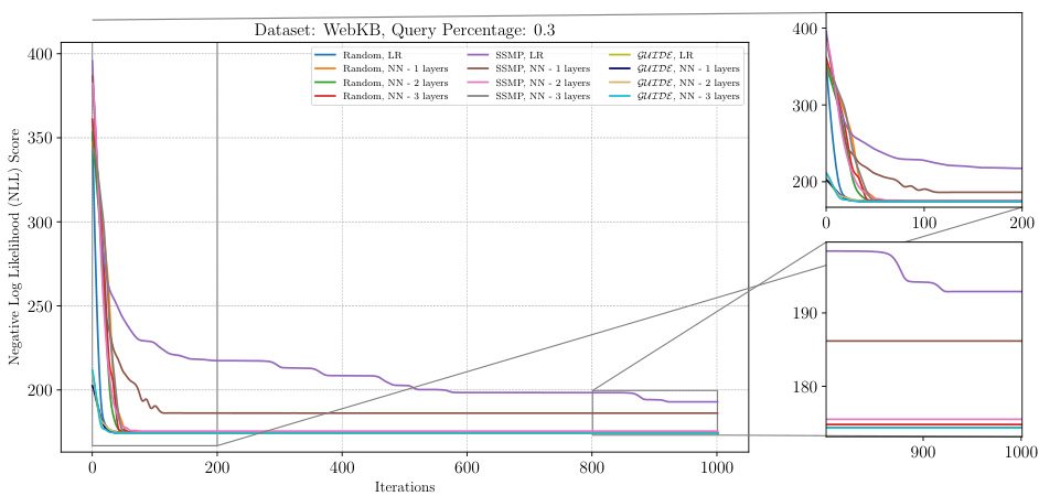
This figure displays the results of the Inference Time Self Supervised Training (ITSELF) algorithm for Probabilistic Circuits (PCs) on the WebKB dataset with a query ratio of 0.1. The graph shows the negative log-likelihood loss across various pre-trained models (Random, SSMP, GUIDE) with different numbers of layers in the neural network. The purpose is to compare the loss values across different model initializations (random, SSMP, GUIDE) and different network architectures to demonstrate the efficacy of the ITSELF algorithm in converging to a near-optimal solution regardless of the initialization. The zoomed-in portions provide more detail on initial and later stages of the optimization.
This figure presents the results of the Inference Time Self Supervised Training (ITSELF) algorithm across various pre-trained models for Probabilistic Circuits (PCs) on the WebKB dataset, specifically focusing on a query ratio of 0.5. The plot shows the negative log-likelihood (NLL) loss against the number of iterations. Different lines represent different model initialization strategies (random, SSMP, and GUIDE) with varying numbers of hidden layers (1, 2, or 3). The figure helps to compare the convergence speed and final loss achieved by these different initialization strategies and network architectures. The zoomed-in plots (lower panels) provide a detailed look at the loss convergence during the early and later stages of the ITSELF process.
This figure shows the negative log-likelihood loss across different training methods (Random, SSMP, GUIDE) and network architectures (LR, NN with 1, 2, or 3 layers) for PCs on the WebKB dataset at a query ratio of 0.1, using the ITSELF algorithm. The main plot displays the loss over 1000 iterations. The subplots provide a zoomed-in view of the first 200 and last 200 iterations, highlighting convergence behavior and loss stability for various models.
The figure shows the negative log-likelihood loss values over 1000 iterations of the ITSELF algorithm for PCs on the WebKB dataset with a query ratio of 0.1. Different pre-trained models are used for initialization, namely, models trained with random initialization, SSMP, and GUIDE. Each model uses different numbers of hidden layers in its architecture. The plot clearly illustrates that the GUIDE pre-trained models consistently converge to lower loss values than others, demonstrating their superior performance in this specific scenario.
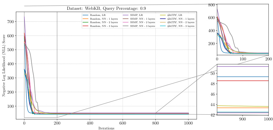
This figure shows the results of the ITSELF algorithm, which iteratively refines the MPE solution during inference, for PCs on the Reuters-52 dataset with a query ratio of 0.9. The plot displays the negative log likelihood loss across different training methods (Random, SSMP, GUIDE) and network architectures (LR, 1-3 hidden layers) over 1000 iterations. The zoomed-in subplots show the initial and final convergence behavior. The figure demonstrates the different convergence rates and final loss values across methods highlighting the effect of pre-training and network architecture.
The figure shows the results of the ITSELF algorithm (Inference Time Self-Supervised Training) applied to Neural Autoregressive Models (NAMs) on the DNA dataset with a query ratio of 0.5. The x-axis represents the number of iterations of the ITSELF algorithm, and the y-axis represents the negative log-likelihood (NLL) score. Different colored lines represent various pre-trained models (Random, SSMP, and GUIDE) with different numbers of layers in the neural network architecture. The zoomed-in plots show the convergence details during the initial and final stages of ITSELF’s optimization.
This figure displays the results of the Inference Time Self Supervised Training (ITSELF) algorithm’s performance across different pre-trained models for Neural Autoregressive Models (NAMs) on the DNA dataset with a query ratio of 0.5. The graph shows how the negative log likelihood (NLL) score changes over 1000 iterations of the ITSELF algorithm. The different lines represent different pre-training methods: random initialization with linear and 1-3 hidden layers, SSMP (Self-Supervised MPE) pre-training with linear and 1-3 hidden layers, and GUIDE pre-training with linear and 1-3 hidden layers. The zoomed-in plots highlight the performance in the first and last 200 iterations, revealing convergence patterns and differences among methods.
The figure shows the result of applying the ITSELF algorithm to Neural Autoregressive Models (NAMs) on the DNA dataset with a query ratio of 0.5. Different initialization methods are compared: random initialization with different numbers of layers in the neural network, SSMP (Self-Supervised MPE), and GUIDE (Guided Iterative Dual Learning). The plot shows the negative log likelihood (NLL) score over 1000 iterations of the ITSELF algorithm. The zoomed in sections highlight the behaviour during the initial and final iterations.
This figure shows the negative log-likelihood loss values for different pre-trained models (Random, SSMP, GUIDE) using various architectures (LR, NN with 1, 2, and 3 layers) during the ITSELF optimization process on the Reuters-52 dataset. The x-axis represents the number of iterations, and the y-axis shows the loss value. The plot illustrates how the loss changes over iterations for different initialization methods and network complexities, allowing for comparison of convergence speed and final loss.
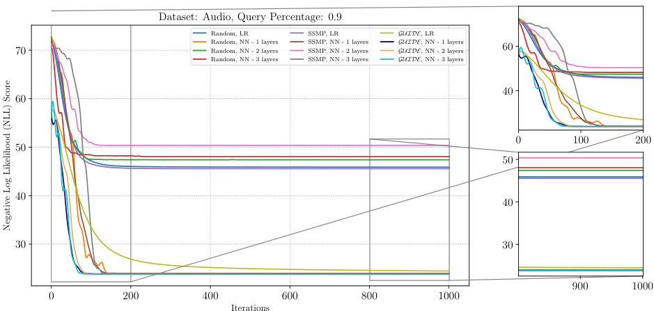
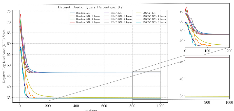
The figure shows the negative log-likelihood loss values over 1000 iterations of ITSELF for PCs on the Audio dataset with a query ratio of 0.7. Multiple lines represent different initialization strategies: random initialization with different numbers of layers in the neural network, SSMP (Self-Supervised MPE) initialization with various layer counts, and GUIDE (Guided Iterative Dual Learning with Self-Supervised Teacher) initialization with different layer counts. The plot helps to illustrate the convergence behavior of ITSELF under different initialization schemes and layer depths. The subplots zoom in on the initial and final 200 iterations for a more detailed analysis of convergence patterns.
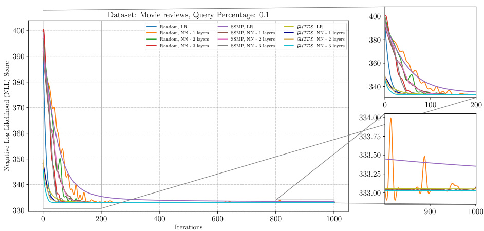
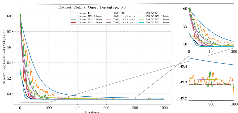
This figure displays the negative log-likelihood loss across various pre-trained models for probabilistic circuits (PCs) on the Netflix dataset at a query ratio of 0.3. The x-axis represents the number of ITSELF iterations, and the y-axis represents the negative log-likelihood loss. The plot shows the loss curves for different initialization methods: Random (with different numbers of layers), SSMP, and GUIDE. Each line represents a different model configuration. The subplots offer a zoomed-in view of the loss during initial and final iterations of ITSELF.
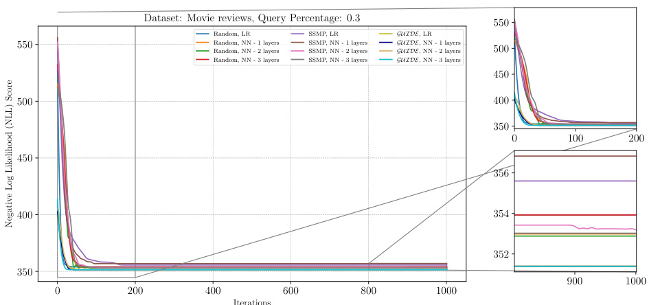
The figure shows the Negative Log Likelihood (NLL) loss for different PC models trained with various methods (random, SSMP, GUIDE) over 1000 ITSELF iterations. The plot displays the NLL loss for different models with 1,2, and 3 layers. It illustrates how the choice of pre-training method and network architecture impacts the convergence of the ITSELF algorithm. A zoomed-in view of the initial and final 200 iterations is also provided for a more detailed analysis.
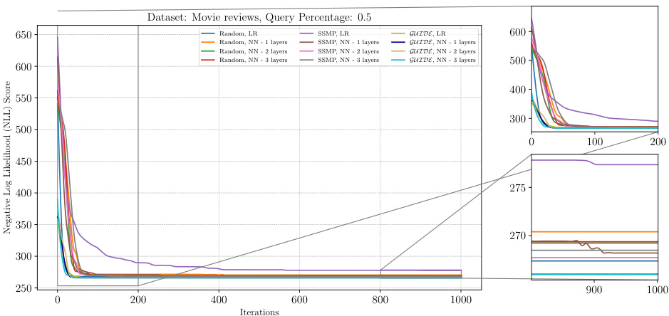
This figure shows the analysis of the ITSELF loss across different pre-trained models for probabilistic circuits (PCs) on the Netflix dataset with a query ratio of 0.3. The x-axis represents the number of ITSELF iterations, and the y-axis shows the negative log-likelihood (NLL) score. Multiple lines are shown, each representing a different model initialization (random, SSMP, and GUIDE), and different numbers of layers in the neural network architecture. The zoomed-in plots show the initial and final portions of the curves to better illustrate the convergence behavior of the various models. The figure illustrates that models pre-trained with the GUIDE approach generally converge to lower loss values more quickly than those initialized with the SSMP or randomly initialized methods. This showcases the effectiveness of the proposed two-phase pre-training strategy of GUIDE.
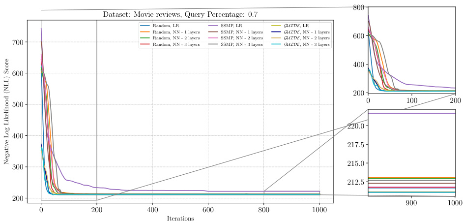
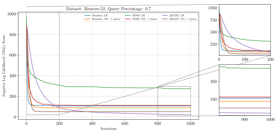
This figure shows the negative log-likelihood loss values over 1000 iterations of the ITSELF algorithm for different pre-trained models (random initialization, SSMP, and GUIDE) on the Reuters-52 dataset with a query ratio of 0.7. The plots show the impact of different pre-training methods on the convergence speed and final loss value of the ITSELF algorithm. Each line represents a different model, and the plot helps to understand the benefits of the GUIDE pre-training method compared to other approaches.
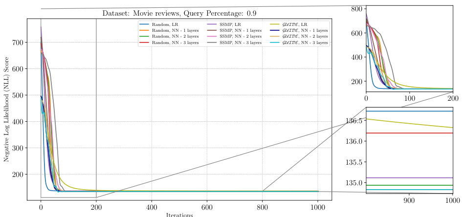
This figure shows the negative log-likelihood loss over 1000 iterations of ITSELF for various pre-trained models (random initialization, SSMP, GUIDE) and different neural network architectures (LR, NN with 1, 2 and 3 layers). The results are for the Reuters-52 dataset with a query ratio of 0.9. The plot shows how the loss changes iteratively during inference time using the ITSELF algorithm for different pre-training techniques and model complexities. It allows to compare the efficacy of different model initializations and architectures in solving the MPE task within this specific dataset and query ratio.
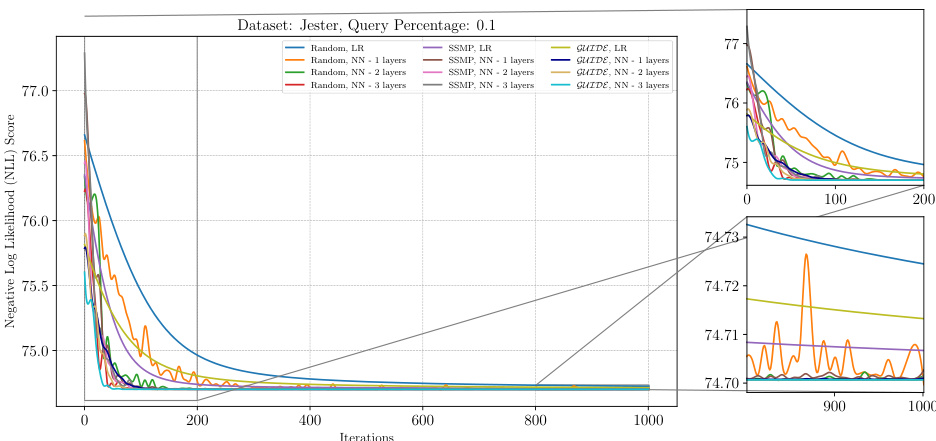
The figure shows the analysis of the ITSELF loss across various pre-trained models for Neural Autoregressive Models (NAMs) on the DNA dataset at a query ratio of 0.5. It compares different initialization methods (Random, SSMP, and GUIDE) using both LR (logistic regression) and NN (neural network) architectures with varying numbers of layers. The x-axis represents the number of iterations, and the y-axis represents the negative log likelihood (NLL) score, which is a measure of the model’s performance. The plots show how the loss changes over multiple iterations, indicating how the different initialization methods affect the convergence and final performance of the ITSELF algorithm.
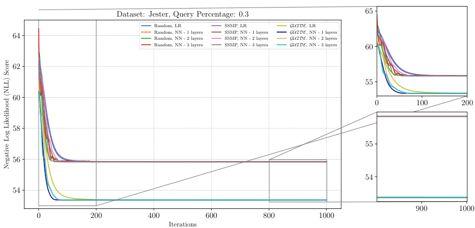
The figure shows the negative log-likelihood loss over 1000 iterations of ITSELF for various pre-trained models on the Netflix dataset with a query ratio of 0.3. The pre-trained models include those initialized randomly, using the SSMP method, and using the GUIDE method. Each model is evaluated with different numbers of hidden layers (1, 2, or 3). The plot shows that models pre-trained with GUIDE generally have a better starting point (lower loss) for ITSELF compared to the other methods.
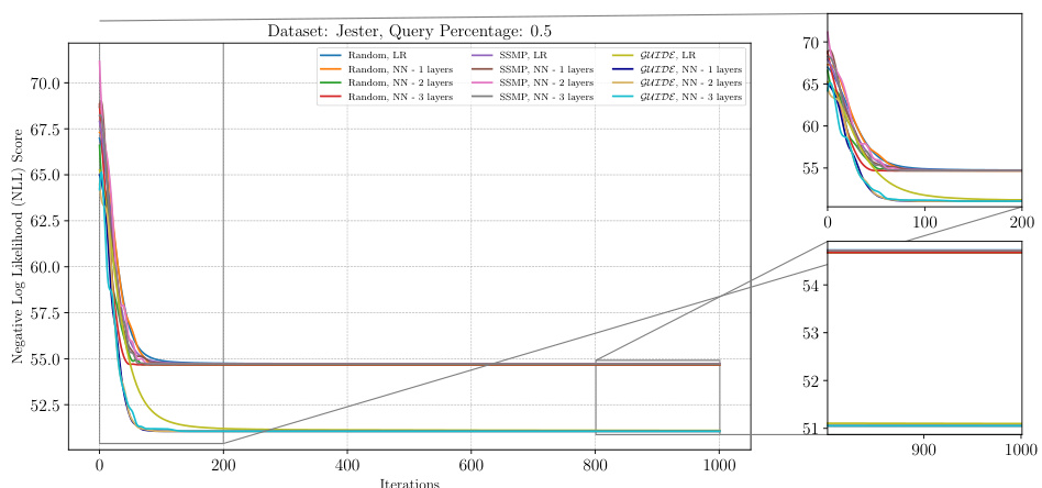
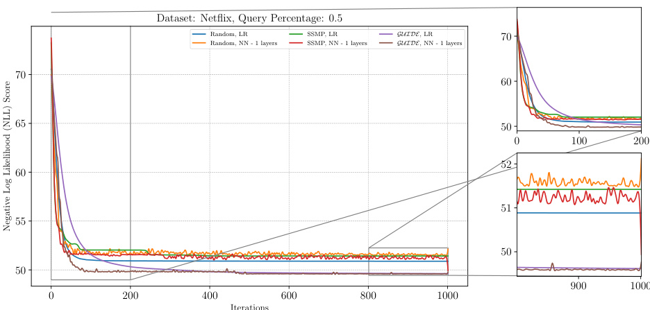
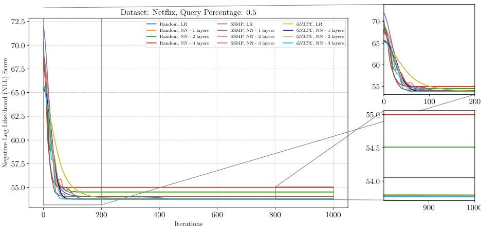
This figure presents a detailed analysis of the ITSELF (Inference Time Self Supervised Training) algorithm’s performance across various pre-trained models for Probabilistic Circuits (PCs) on the Netflix dataset, specifically focusing on a query ratio of 0.5. The x-axis represents the number of iterations of the ITSELF algorithm, and the y-axis shows the negative log-likelihood (NLL) score, a measure of model performance. Different colored lines represent different model types and pre-training methods including those using Random initialization, SSMP (Self-Supervised MPE), and GUIDE (Guided Iterative Dual Learning). The zoomed-in views provide finer-grained insights into early and late stages of the optimization process. The figure helps to illustrate the convergence behavior of ITSELF under various initialization techniques and model architectures.
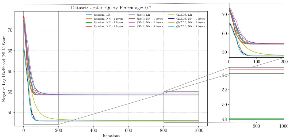
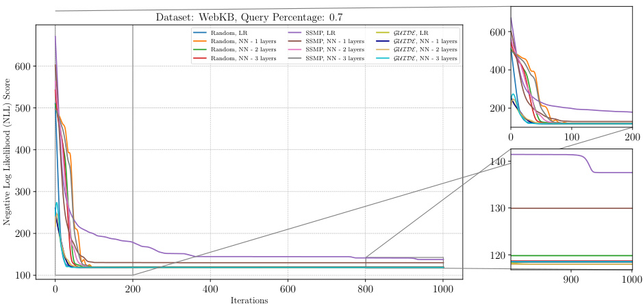
The figure shows the analysis of ITSELF loss across various pre-trained models for Neural Autoregressive Models (NAMs) on the WebKB dataset at a query ratio of 0.7. The graph plots the negative log-likelihood loss (NLL) against the number of ITSELF iterations. Different lines represent different pre-training methods (Random, SSMP, GUIDE) and different neural network architectures (LR - linear regression, NN - neural networks with varying numbers of layers). The zoomed-in subplots on the right allow for a clearer view of early and late stages of ITSELF optimization.
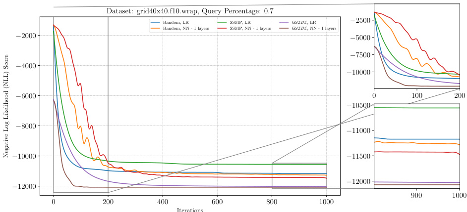
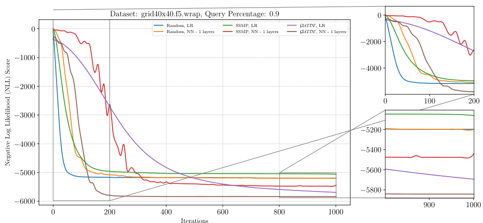
The figure shows the analysis of the ITSELF loss across various pre-trained models for PGMs on the grid40x40.f10.wrap dataset at a query ratio of 0.7. The main plot displays the negative log-likelihood loss over 1000 iterations, comparing different initialization methods (Random, SSMP, GUIDE) and network architectures (LR, NN-1 layers). The insets provide a zoomed-in view of the first 200 and last 200 iterations to highlight early and late convergence behavior. Each line represents a different model configuration, demonstrating how initialization and architecture impact training performance.
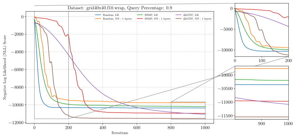
This figure shows the negative log-likelihood loss for different models trained with different methods (Random, SSMP, GUIDE) across 1000 iterations of ITSELF. The results are presented for a specific dataset (grid40x40.f10.wrap) and query ratio (0.9). The figure helps to understand the convergence behavior of different models during inference time optimization using self-supervised loss. The zoomed-in plots shows the initial and final 200 iterations more clearly.
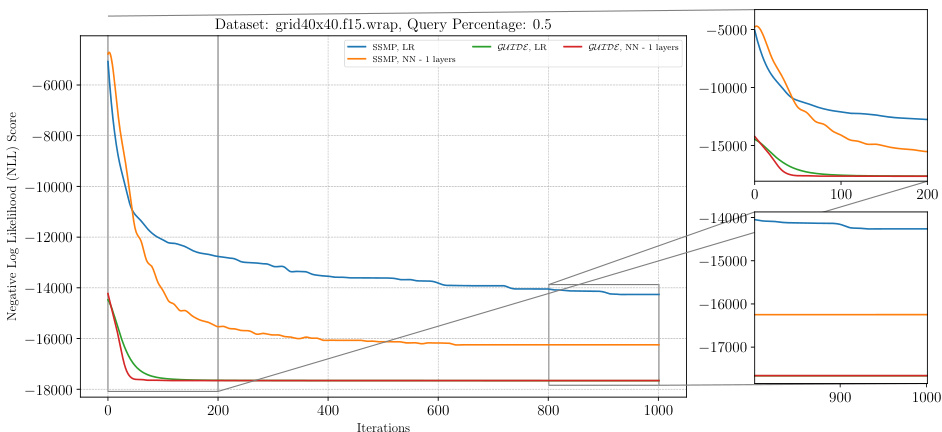
This figure displays the negative log-likelihood loss over 1000 iterations of the ITSELF algorithm. Six different models are compared, each initialized with one of three different pre-training methods (Random, SSMP, GUIDE) combined with either a logistic regression layer or a 1-layer neural network. The plot shows that models pre-trained using the GUIDE method generally have a better starting point and converge to a lower loss compared to the other models.
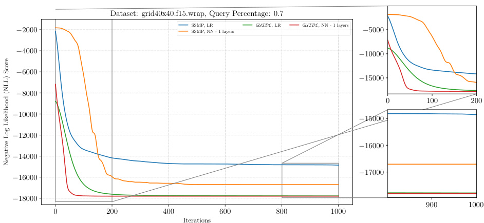
This figure displays the negative log-likelihood (NLL) loss over 1000 iterations of the ITSELF algorithm for various pre-trained models on the grid40x40.f15.wrap dataset of PGMs, at a query ratio of 0.7. The plot shows the convergence of the loss over time. The different lines represent different model initializations (random, SSMP, and GUIDE) and different network architectures (LR and NN with 1 hidden layer). The zoomed-in subplots show the first 200 and last 200 iterations for better visualization of the convergence behavior.
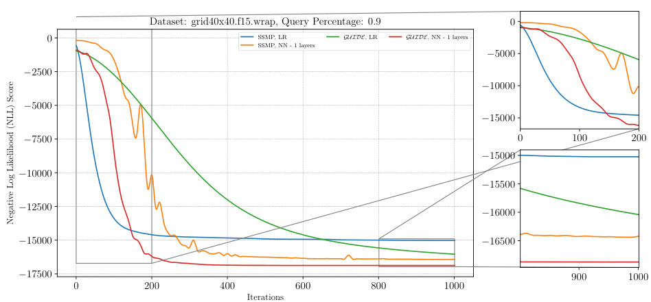
This figure displays the negative log-likelihood loss over 1000 iterations of ITSELF for different pre-trained models (Random, SSMP, GUIDE) on a PGM dataset (grid40x40.f15.wrap) with a query ratio of 0.9. Each line represents a different model with either a linear regression (LR) or a neural network with one hidden layer (NN-1 layers). The plot shows the model’s convergence progress toward the minimum loss value.
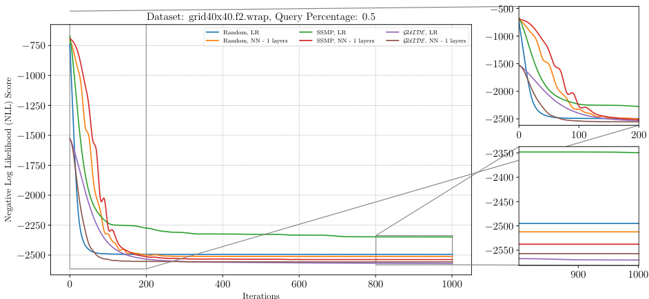
The figure shows the negative log-likelihood loss for various pre-trained models for PGMs (probabilistic graphical models) on the grid40x40.f2.wrap dataset at a query ratio of 0.5 using the ITSELF (Inference Time Self Supervised Training) method. The x-axis represents the number of iterations and the y-axis shows the negative log-likelihood loss score. Different colors represent different models: Random with linear regression (LR), Random with neural networks (NN) of 1, 2, and 3 layers, SSMP (Self-Supervised Neural Network Approximator for MPE) with LR and NN, and GUIDE (Guided Iterative Dual LEarning with Self-supervised Teacher) with LR and NN. The smaller subplots on the right show a zoomed-in view of the loss curves at the beginning (0-200 iterations) and end (900-1000 iterations) of training. The plot demonstrates the performance of different pre-training methods combined with ITSELF during inference, showcasing the advantages of the proposed methods.
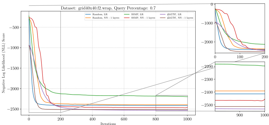
This figure shows the negative log-likelihood (NLL) loss over 1000 ITSELF iterations for various pre-trained models on the grid40x40.f2.wrap dataset with a query ratio of 0.5. The plot compares models initialized randomly (with and without a single hidden layer) and pre-trained using SSMP and GUIDE (again, both with and without a single hidden layer). The zoomed-in plots on the right show the initial and final 200 iterations, respectively, highlighting the convergence behavior and the differences in initial loss among different model training methods.
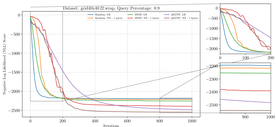
The figure shows the performance of the ITSELF algorithm for solving the Most Probable Explanation (MPE) query on a probabilistic graphical model (PGM) dataset. The x-axis represents the number of ITSELF iterations, and the y-axis represents the negative log-likelihood (NLL) score. Different lines represent different pre-trained models: Random, SSMP, and GUIDE, each with and without additional neural network layers. The plot shows how the loss (and thus the quality of the MPE solution) changes with more iterations for each model. The inset plots provide close-ups of the early and later stages of training to better show the details of convergence behavior.
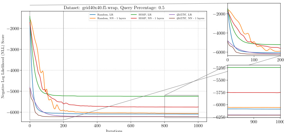
The figure shows the negative log-likelihood loss across different iterations of ITSELF algorithm for PGMs on the grid40x40.f15.wrap dataset at a query ratio of 0.5. Different lines represent various pre-trained models (Random, SSMP, GUIDE) with different numbers of layers. The plot shows the convergence behavior of the loss function for each model during the inference process. It helps to understand the efficacy and convergence speed of various models.
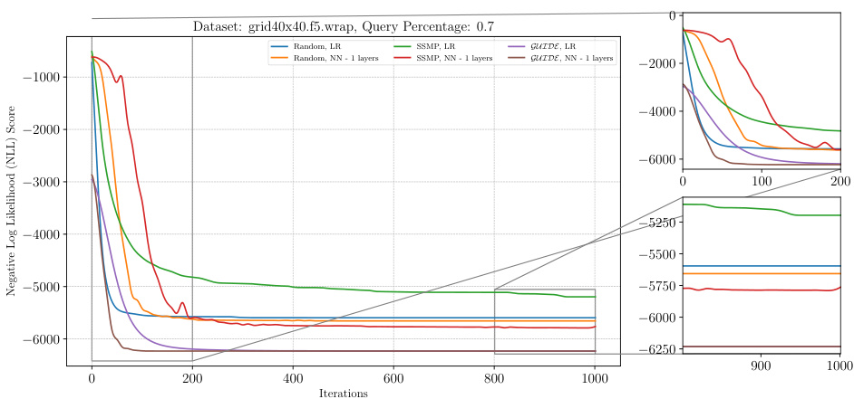
The figure shows the negative log-likelihood loss during the ITSELF (Inference Time Self-Supervised Training) process for different pre-trained models on a Probabilistic Graphical Model (PGM) dataset. The x-axis represents the number of ITSELF iterations, and the y-axis shows the negative log-likelihood loss. Different colored lines represent different model pre-training methods (Random, SSMP, GUIDE) and network architectures (LR - linear regression, 1 layer neural network). The inset shows a zoomed-in view of the convergence phase, highlighting the differences in the final loss achieved by various models. The main plot shows how quickly each pre-training method converges to a minimum loss value.
The figure shows the negative log-likelihood loss across different iterations for various pre-trained models of Probabilistic Graphical Models (PGMs) on the grid40x40.f15.wrap dataset at a query ratio of 0.9. The x-axis represents the number of iterations, and the y-axis represents the negative log-likelihood (NLL) loss. Different colored lines represent different pre-trained models, allowing for a comparison of their performance in minimizing the loss. The zoomed in plots show the details of the convergence behavior.
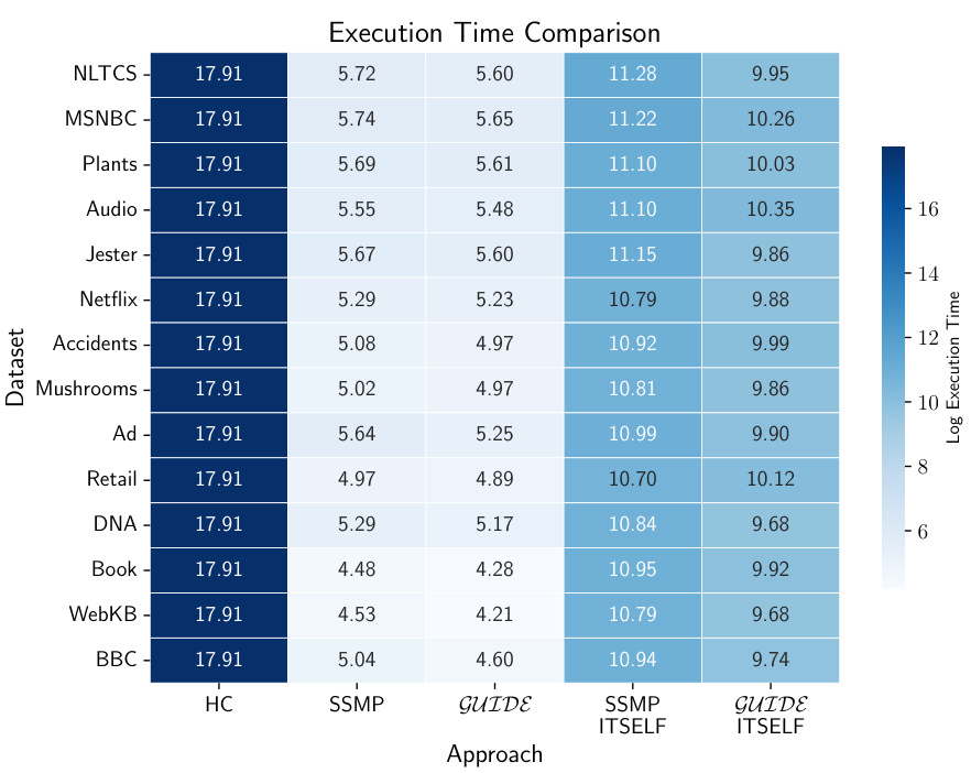
The figure is a heatmap visualizing inference time for MADE models across various datasets and different inference approaches (HC, SSMP, GUIDE, SSMP+ITSELF, GUIDE+ITSELF). Lighter colors represent faster inference times. The heatmap allows for a quick comparison of inference speed between different methods on different datasets, illustrating the impact of each technique on computational efficiency.
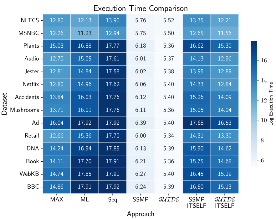
This heatmap visualizes the inference times of different methods for MADE models across various datasets. Each cell represents the inference time in microseconds on a logarithmic scale. The color intensity corresponds to inference time, with lighter colors representing faster inference. The heatmap allows for a quick comparison of the relative speeds of different approaches.
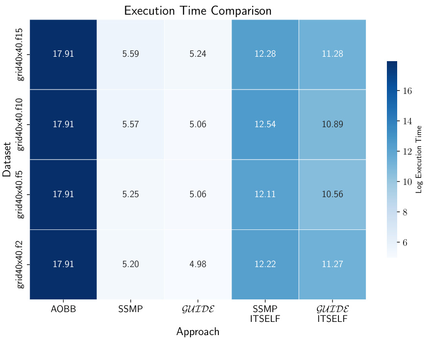
This heatmap visualizes the inference times for different probabilistic graphical models (PGMs) using various approaches. The rows represent four different PGM datasets (grid40x40.f2, grid40x40.f5, grid40x40.f10, and grid40x40.f15), and the columns represent five different inference methods: AOBB, SSMP, GUIDE, SSMP+ITSELF, and GUIDE+ITSELF. Each cell’s color intensity indicates the log of the inference time in microseconds, with lighter colors representing faster inference times. This figure allows for a quick comparison of the relative efficiency of different methods across various PGM datasets.
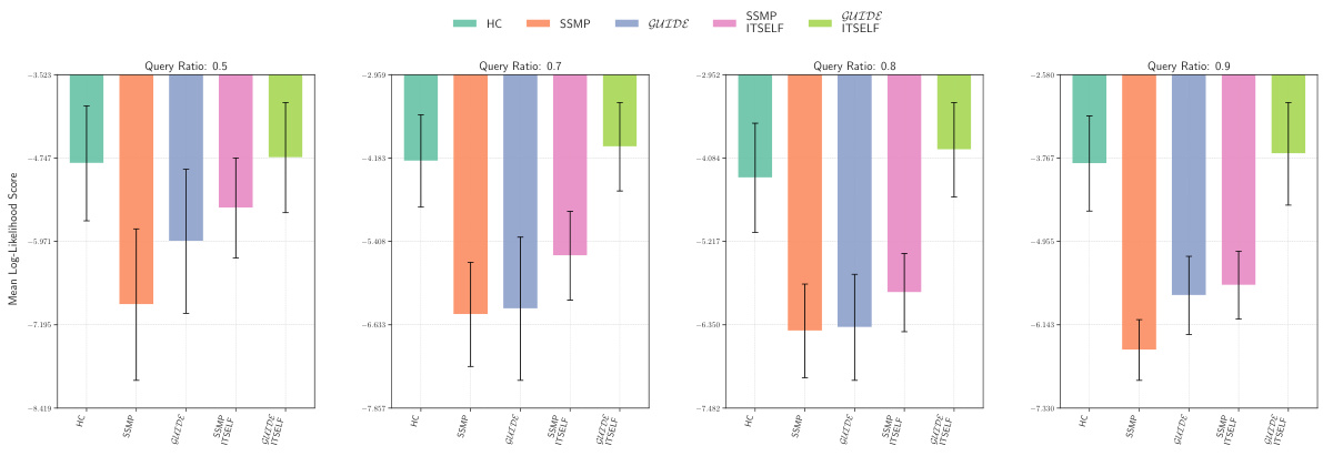
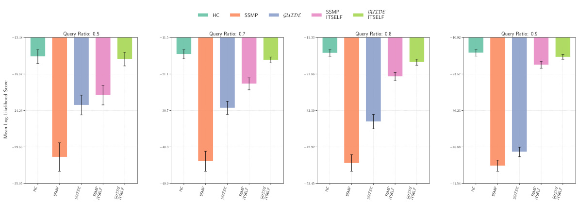
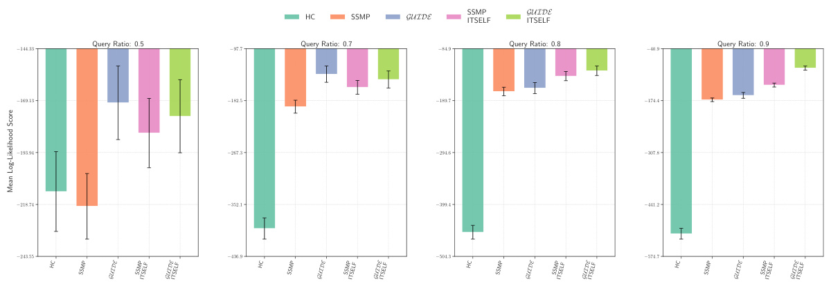
This figure displays the mean log-likelihood scores for different methods on the NLTCS dataset for Neural Autoregressive Models (NAMs). Each bar represents the average log-likelihood score for a specific method (HC, SSMP, GUIDE, SSMP+ITSELF, and GUIDE+ITSELF), with error bars indicating the standard deviation. The query ratio varies across the columns (0.5, 0.7, 0.8, 0.9). Higher scores indicate better performance.
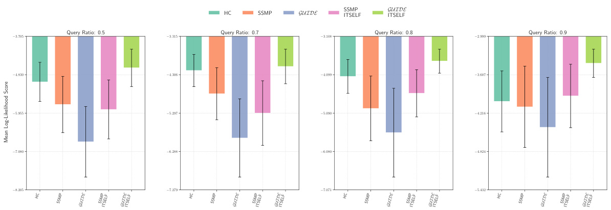
This figure displays the mean log-likelihood scores for different methods (HC, SSMP, GUIDE, SSMP+ITSELF, GUIDE+ITSELF) across various query ratios (0.5, 0.7, 0.8, 0.9) for the NLTCS dataset using Neural Autoregressive Models (NAMs). Error bars represent the standard deviation. Higher scores indicate better performance, showing the effectiveness of the ITSELF optimization and the GUIDE pre-training method.
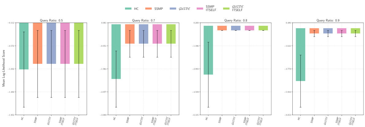
This figure displays the performance of different methods for solving the Most Probable Explanation (MPE) task on the NLTCS dataset using Neural Autoregressive Models (NAMs). Each bar represents the mean log-likelihood score (+/- standard deviation) for a given method across various query ratios. Higher scores indicate better performance. The methods compared are Hill Climbing (HC), SSMP, GUIDE, SSMP + ITSELF, and GUIDE + ITSELF.
This figure presents two heatmaps visualizing the percentage difference in mean log-likelihood (LL) scores between the proposed GUIDE + ITSELF method and a baseline method (MAX for PCs, HC for NAMs). The heatmaps effectively showcase the performance gains of the proposed approach across various datasets and query ratios. Green cells indicate superior performance of GUIDE + ITSELF, while darker shades represent a larger percentage difference, highlighting the impact of increasing problem complexity.
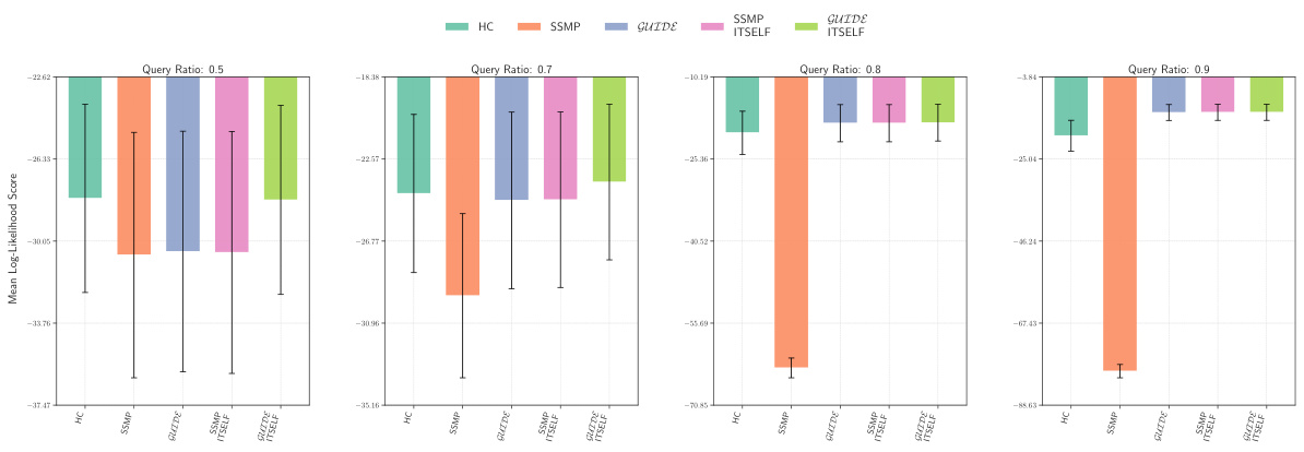
This figure displays the log-likelihood scores for different methods (HC, SSMP, GUIDE, SSMP+ITSELF, GUIDE+ITSELF) on the NLTCS dataset for Neural Autoregressive Models (NAMs). The x-axis represents different query ratios, and the y-axis represents the mean log-likelihood score. Error bars indicate standard deviation. Higher scores indicate better performance, showing the relative effectiveness of each method at various query ratios.
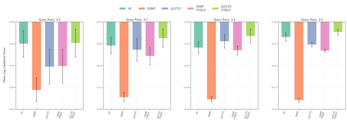
This figure displays the mean log-likelihood scores for different methods (HC, SSMP, GUIDE, SSMP + ITSELF, GUIDE + ITSELF) on the NLTCS dataset for Neural Autoregressive Models (NAMs). The x-axis represents different query ratios (the fraction of variables considered as query variables), and each bar represents the average log-likelihood score for a given method. Error bars show the standard deviations. Higher scores indicate better performance, reflecting the effectiveness of the proposed methods (GUIDE, ITSELF) in maximizing log-likelihood compared to baselines (HC, SSMP).
This figure presents a comparison of log-likelihood scores for different methods (HC, SSMP, GUIDE, SSMP+ITSELF, GUIDE+ITSELF) on the NLTCS dataset for Neural Autoregressive Models (NAMs). The scores are shown for various query ratios (0.5, 0.7, 0.8, and 0.9), allowing for a comprehensive analysis of the performance of each method across different query sizes. Higher scores indicate better performance.
This figure presents heatmaps visualizing the percentage difference in mean log-likelihood (LL) scores between the proposed GUIDE+ITSELF method and the MAX baseline for Probabilistic Circuits (PCs) and Neural Autoregressive Models (NAMs). The y-axis represents datasets categorized by variable count, and the x-axis shows the query ratio. Each cell’s color intensity indicates the percentage difference in mean LL scores, with green shades indicating superiority of the proposed method and darker shades representing larger differences. The top heatmap shows the results for PCs, and the bottom heatmap shows the results for NAMs. The figure helps to visually compare the performance of the two methods across different datasets and query ratios.
The figure is a heatmap showing inference time for MADE models across various datasets and query ratios. Different neural network training methods (SSMP, GUIDE, and their combinations with ITSELF) are compared to baselines (HC). Lighter colors represent faster inference times.

This figure presents a comparison of different MPE (Most Probable Explanation) methods across various probabilistic models (PMs). The results are displayed in four contingency tables, one each for Probabilistic Circuits (PCs), PCs with hill climbing initialization, Neural Autoregressive Models (NAMs), and Probabilistic Graphical Models (PGMs). Each cell (i,j) in a table shows how many times method i outperformed method j across the 120 tests conducted for each PM. Darker blue shades indicate that method i (rows) consistently outperformed method j (columns). Darker red shades suggest the opposite, and lighter shades show that methods performed similarly. This visualization helps to understand the relative performance of different approaches for solving the MPE task across various models.
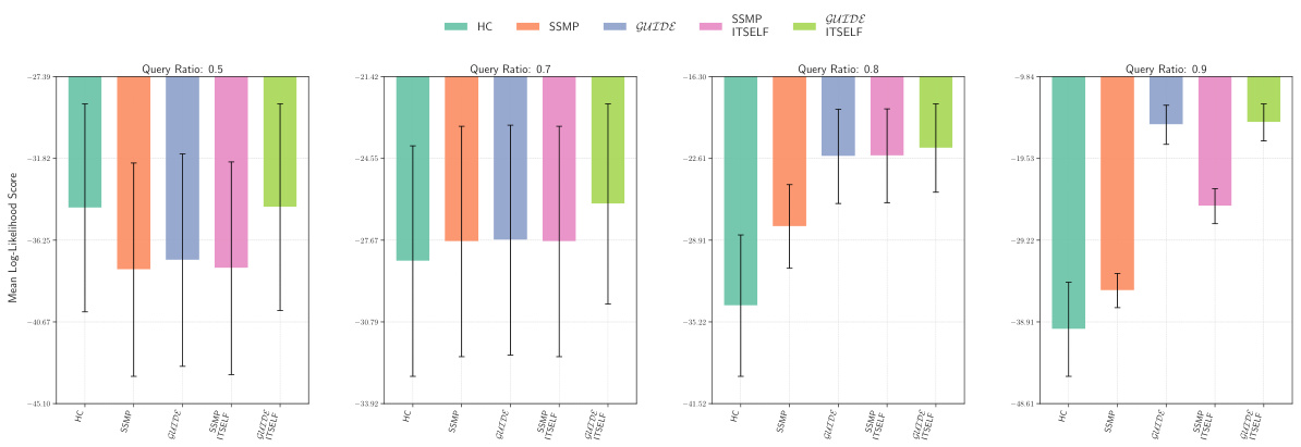
This figure displays the mean log-likelihood scores achieved by different methods (HC, SSMP, GUIDE, SSMP + ITSELF, GUIDE + ITSELF) on the NLTCS dataset for Neural Autoregressive Models (NAMs). The scores are shown for various query ratios (0.5, 0.7, 0.8, and 0.9), illustrating the impact of different training and inference strategies on the model’s performance. Higher scores represent better performance.
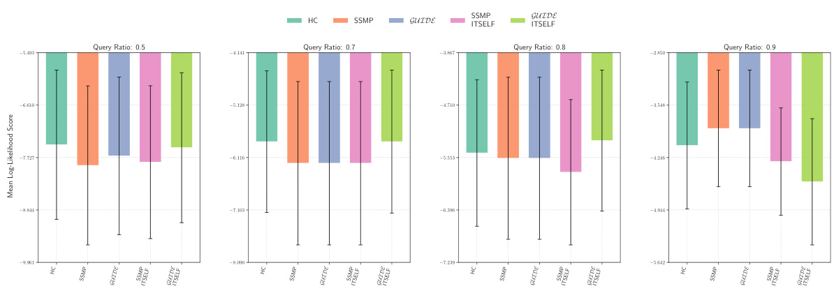
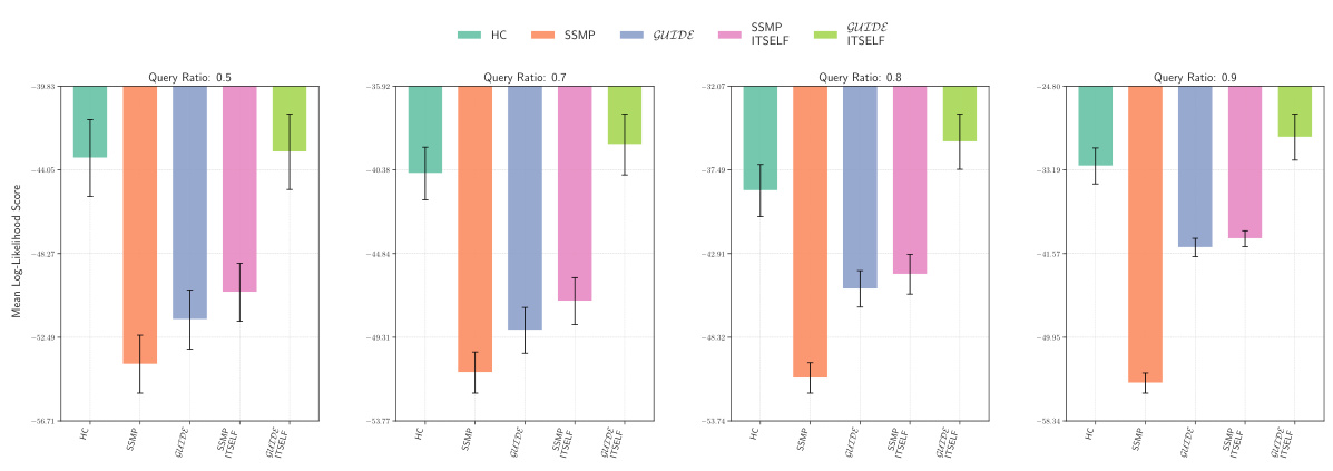
This figure displays the mean log-likelihood scores achieved by different methods on the NLTCS dataset for Neural Autoregressive Models (NAMs). Each group of bars represents a different query ratio (0.5, 0.7, 0.8, 0.9). The bars themselves show the average log-likelihood scores for each method (HC, SSMP, GUIDE, SSMP+ITSELF, GUIDE+ITSELF). Error bars represent the standard deviation. Higher scores indicate better performance, reflecting the effectiveness of the ITSELF (Inference Time Self-Supervised Training) optimization within the GUIDE (Guided Iterative Dual Learning with Self-Supervised Teacher) and SSMP (Self-Supervised Neural Network Approximator for any-MPE) methods.
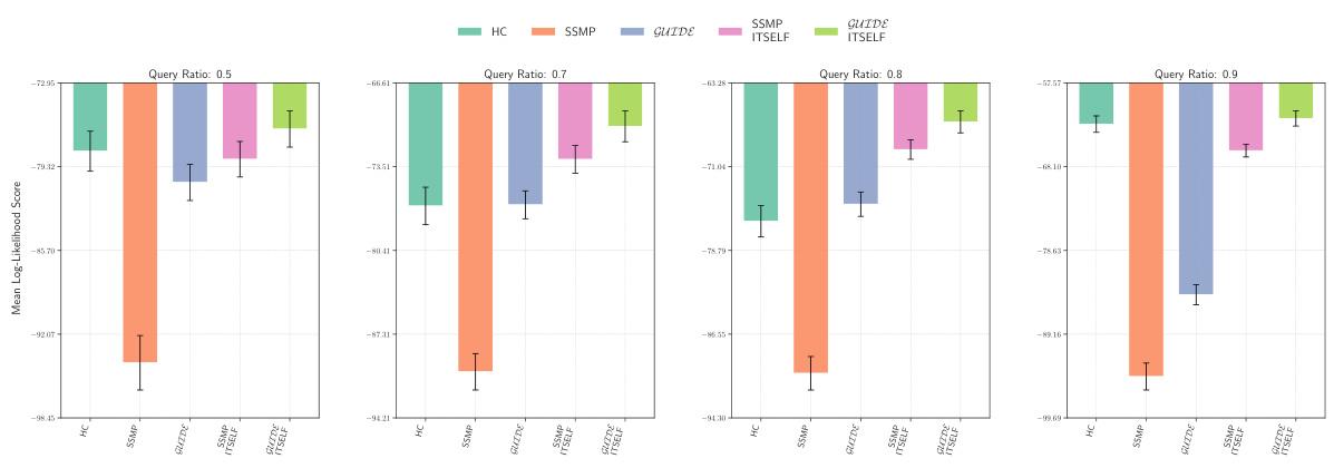
This figure displays the log-likelihood scores for different methods (HC, SSMP, GUIDE, SSMP + ITSELF, GUIDE + ITSELF) on the NLTCS dataset for Neural Autoregressive Models (NAMs). Each bar represents the average log-likelihood score for a particular method across different query ratios (0.5, 0.7, 0.8, 0.9). The error bars indicate the standard deviation. Higher scores represent better performance, indicating the effectiveness of each method in accurately predicting the most probable explanation (MPE).
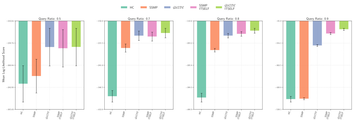
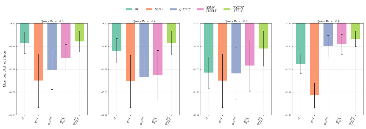
This figure displays the mean log-likelihood scores achieved by different methods (HC, SSMP, GUIDE, SSMP+ITSELF, GUIDE+ITSELF) for the NLTCS dataset across various query ratios. Each bar represents the mean score, and error bars show the standard deviation. Higher scores indicate better performance, reflecting the effectiveness of the proposed methods in accurately predicting the most likely assignment of query variables given the evidence. The figure demonstrates the improvements achieved by incorporating ITSELF inference time optimization and GUIDE two-phase pre-training strategies.
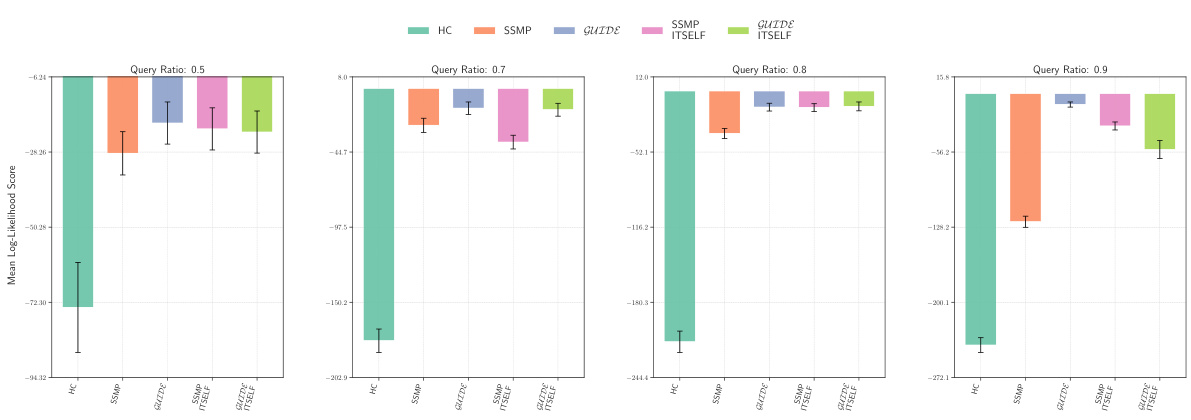
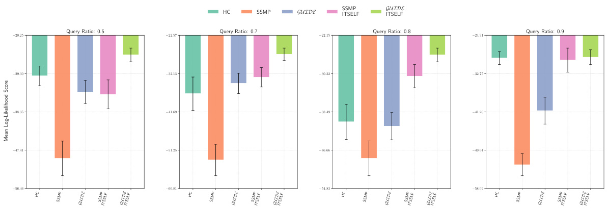
This figure displays the mean log-likelihood scores for different methods (HC, SSMP, GUIDE, SSMP+ITSELF, GUIDE+ITSELF) across various query ratios (0.5, 0.7, 0.8, 0.9) for the NLTCS dataset using Neural Autoregressive Models (NAMs). Each bar represents the mean score for a given method and query ratio, with error bars indicating the standard deviation. Higher scores represent better performance. The figure helps to visually compare the effectiveness of the proposed ITSELF and GUIDE methods against traditional baselines (HC, SSMP) for improving MPE inference accuracy.
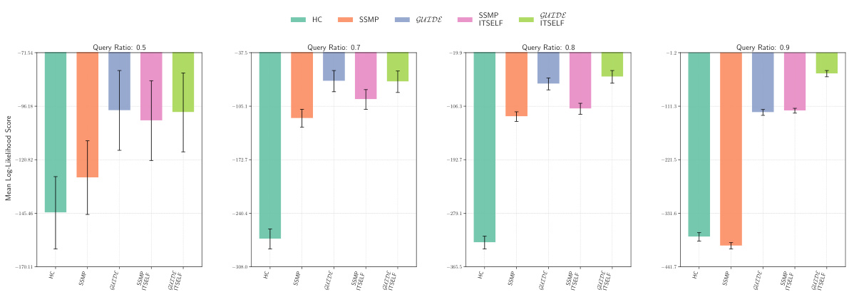
This figure presents two heatmaps that visualize the percentage differences in mean log-likelihood scores between the GUIDE+ITSELF method and the MAX baseline for Probabilistic Circuits (PCs) and Neural Autoregressive Models (NAMs). Each heatmap shows how the performance difference varies across different datasets and query ratios. A green cell indicates that the GUIDE+ITSELF method outperforms the MAX baseline, and a darker shade of green indicates a greater performance difference.
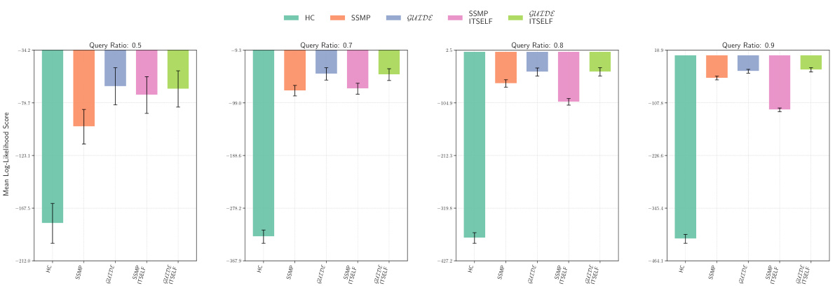
This figure displays the mean log-likelihood scores achieved by different methods (HC, SSMP, GUIDE, SSMP+ITSELF, GUIDE+ITSELF) for the NLTCS dataset across various query ratios (0.5, 0.7, 0.8, 0.9). The bars represent the mean scores, with error bars indicating the standard deviation. Higher scores indicate better performance, reflecting the accuracy of each method in predicting the most probable explanation (MPE).
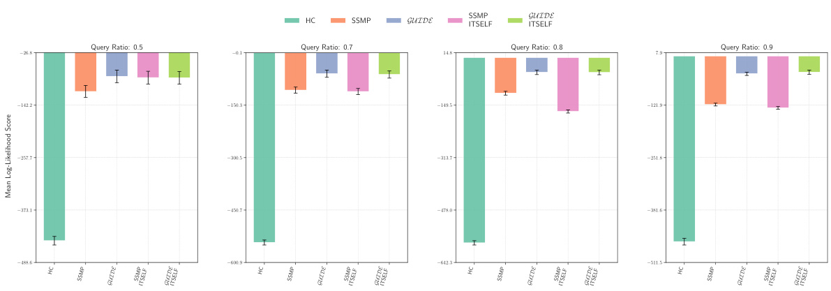
This figure presents a bar chart comparing the performance of different methods (HC, SSMP, GUIDE, SSMP+ITSELF, GUIDE+ITSELF) for solving the Most Probable Explanation (MPE) task on the NLTCS dataset using Neural Autoregressive Models (NAMs). Each bar represents the average log-likelihood score for a specific method, with error bars showing the standard deviation. Higher scores indicate better performance. The chart is divided into sections based on different query ratios (0.5, 0.7, 0.8, 0.9). This figure visually demonstrates the relative effectiveness of the different MPE solution methods across varying query ratios, particularly highlighting the improvement achieved by incorporating the ITSELF optimization technique within the GUIDE training framework.
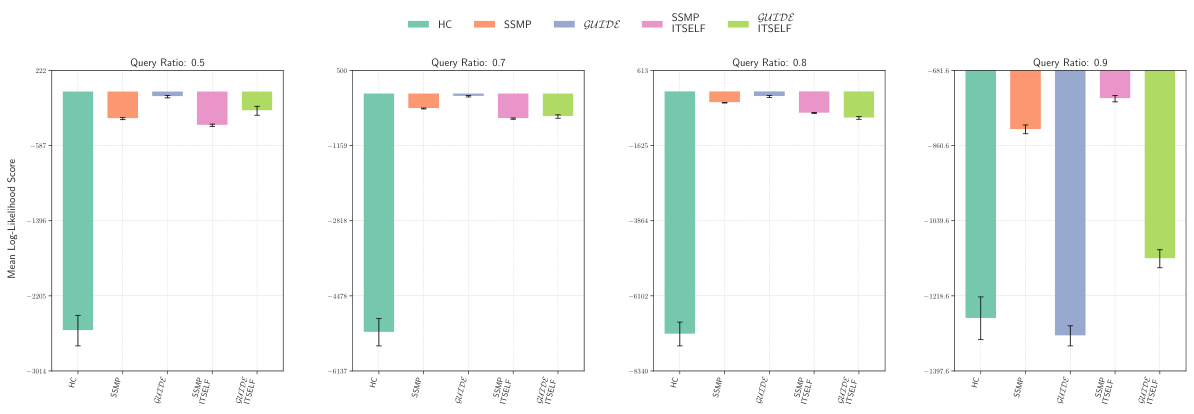
This figure displays the log-likelihood scores for different methods (HC, SSMP, GUIDE, SSMP + ITSELF, GUIDE + ITSELF) across various query ratios (0.5, 0.7, 0.8, 0.9) on the NLTCS dataset for Neural Autoregressive Models (NAMs). Each bar represents the average log-likelihood, with error bars showing the standard deviation. Higher scores indicate better performance, signifying the effectiveness of each method in accurately predicting the most probable explanation (MPE). The plot highlights how the proposed methods (GUIDE and GUIDE + ITSELF) generally outperform other baselines.
This figure presents two heatmaps visualizing the percentage difference in mean log-likelihood (LL) scores between the GUIDE+ITSELF method and the MAX approximation method (top heatmap for PCs and bottom heatmap for NAMs). The x-axis represents the query ratio, while the y-axis shows different datasets. Green cells indicate that GUIDE+ITSELF outperforms MAX, with darker shades representing larger differences. This highlights the superior performance of the proposed method, especially as the dataset size or query complexity increases.
This figure presents contingency tables that compare the performance of various MPE (Most Probable Explanation) methods across different probabilistic models (PMs): Probabilistic Circuits (PCs), Neural Autoregressive Models (NAMs), and Probabilistic Graphical Models (PGMs). Each cell (i, j) in a table shows how often method i outperformed method j across 120 test datasets (for PCs), 80 test datasets (for NAMs), and 16 datasets (for PGMs) using different query ratios. The color intensity indicates the frequency of one method outperforming another. Darker blue means method i frequently outperforms method j, while darker red indicates the opposite. The tables visually summarize the relative strengths and weaknesses of each method across different models and query ratios.
This figure displays the mean log-likelihood scores achieved by different methods (HC, SSMP, GUIDE, SSMP+ITSELF, GUIDE+ITSELF) on the NLTCS dataset for Neural Autoregressive Models (NAMs). The x-axis represents different query ratios, and the y-axis shows the mean log-likelihood score. Error bars indicate the standard deviation. Higher scores suggest better performance, reflecting the effectiveness of the proposed ITSELF and GUIDE methods compared to baselines.
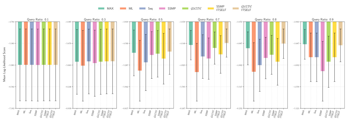
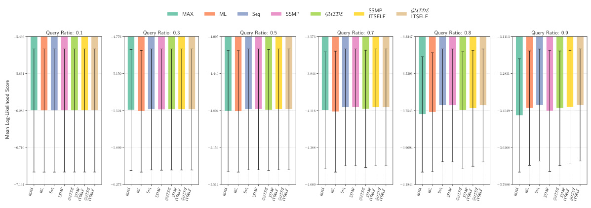
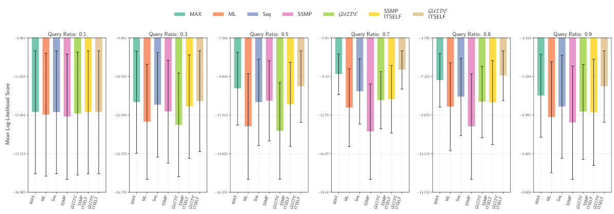
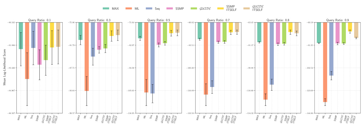
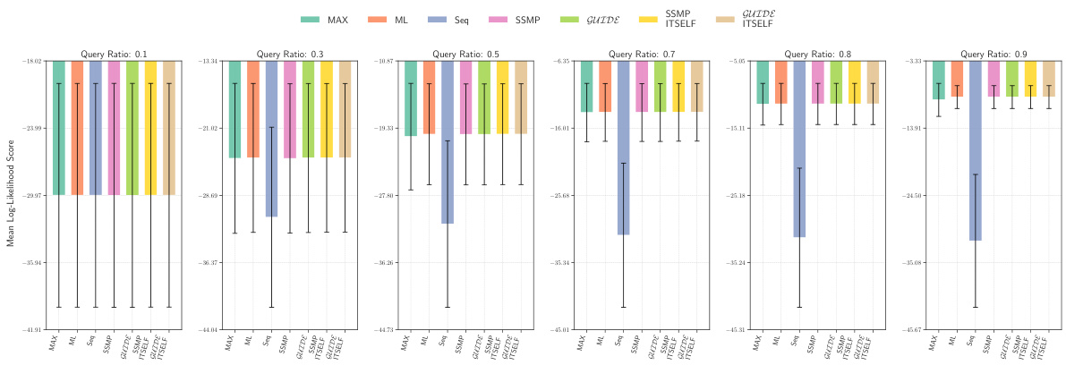
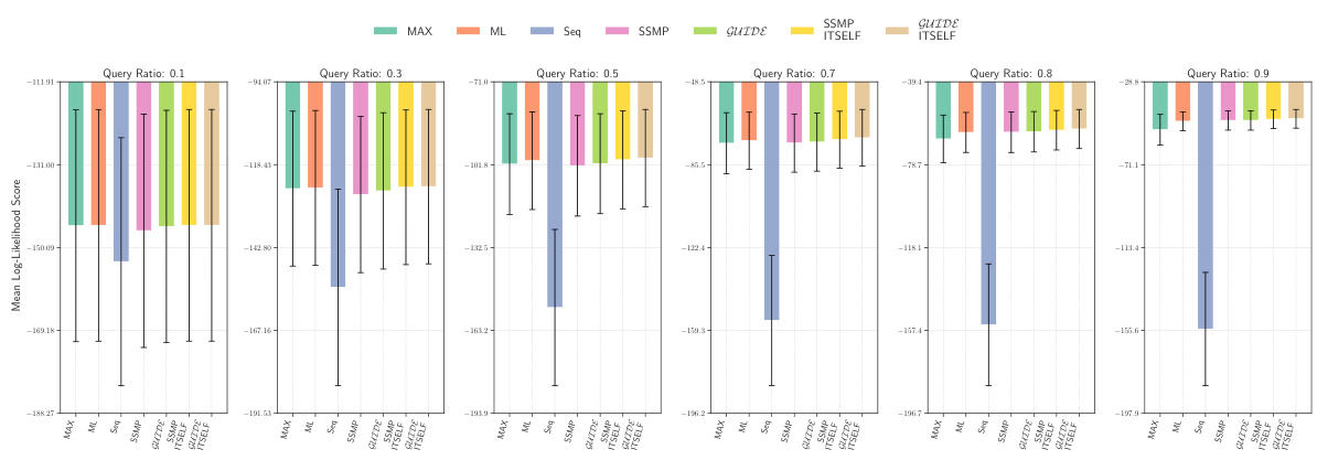
This figure displays the mean log-likelihood scores achieved by different methods (MAX, ML, Seq, SSMP, GUIDE, SSMP + ITSELF, GUIDE + ITSELF) across various query ratios (0.1, 0.3, 0.5, 0.7, 0.8, 0.9) on the Audio dataset using Probabilistic Circuits (PCs). The error bars represent the standard deviation. Higher scores represent better performance. The figure helps in comparing the effectiveness of different approaches in achieving high log-likelihood scores for MPE inference using PCs on this specific dataset.
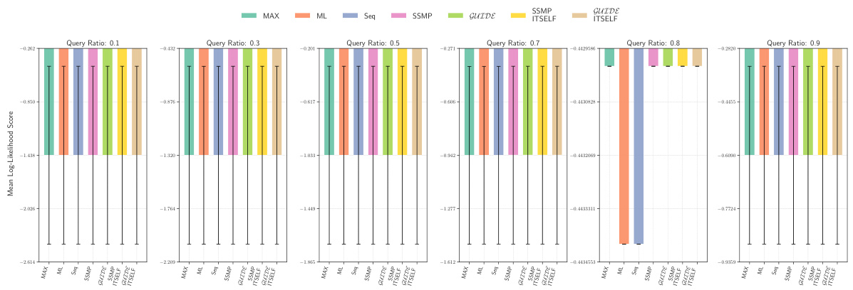
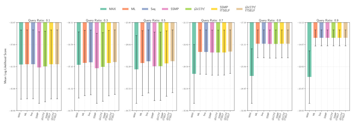
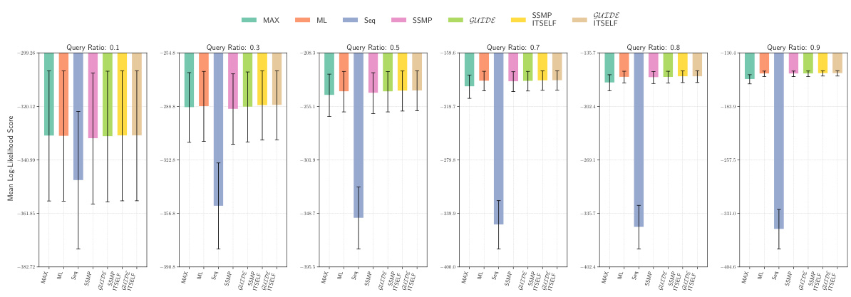
This figure compares the log-likelihood scores across different methods (MAX, ML, Seq, SSMP, GUIDE, SSMP+ITSELF, GUIDE+ITSELF) for the NLTCS dataset at various query ratios (0.1 to 0.9). Each bar represents the mean log-likelihood score with error bars showing the standard deviation. Higher scores represent better performance, indicating the effectiveness of the different approaches for PCs.
This figure presents a comparison of different MPE (Most Probable Explanation) methods across various probabilistic models (PMs). The results are shown in contingency tables for PCs (Probabilistic Circuits), NAMs (Neural Autoregressive Models), and PGMs (Probabilistic Graphical Models). Each cell in the table represents how often one method outperforms another across 120 test datasets. The color of the cells indicates the relative performance of the methods; darker shades represent more significant differences. In general, methods incorporating ITSELF (Inference Time Self Supervised Training) significantly outperform the baselines across all datasets.
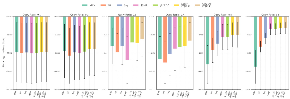
This figure displays the mean log-likelihood scores achieved by different methods (HC, SSMP, GUIDE, SSMP+ITSELF, and GUIDE+ITSELF) for the NLTCS dataset across various query ratios. Error bars representing the standard deviation are included for each. Higher scores indicate better performance, showing the relative effectiveness of each method for this specific dataset. This is part of a larger analysis comparing log-likelihoods across several datasets and models.
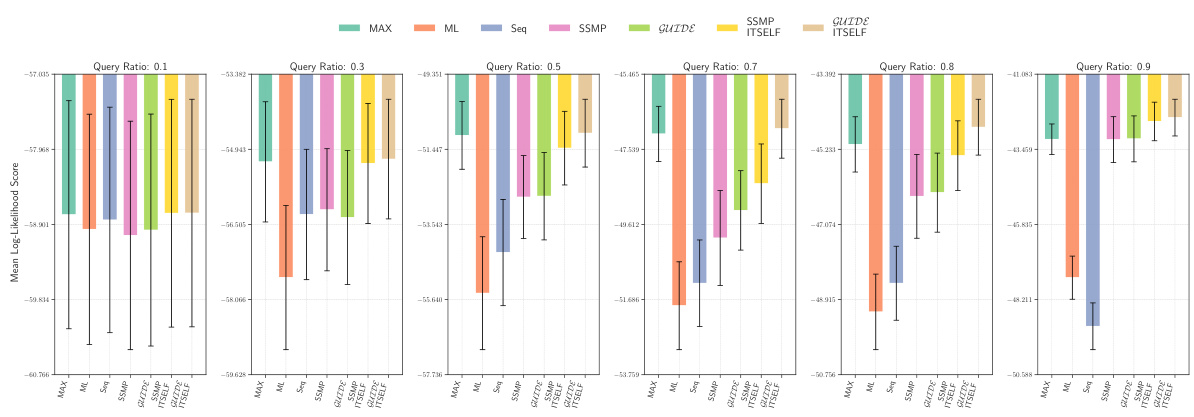
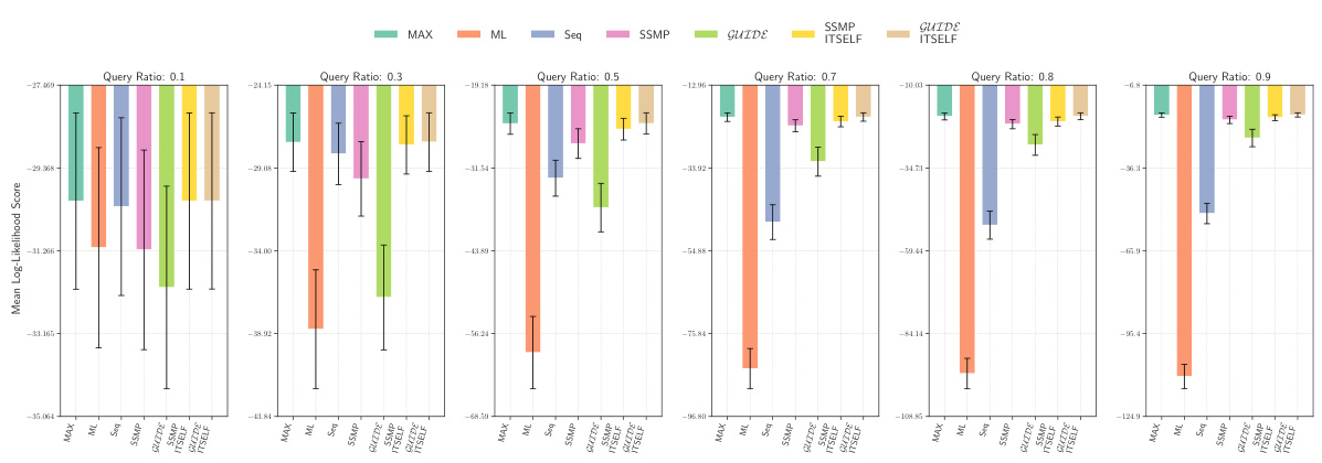
This figure displays the log-likelihood scores for different methods (MAX, ML, Seq, SSMP, GUIDE, SSMP+ITSELF, GUIDE+ITSELF) on the NLTCS dataset for Probabilistic Circuits (PCs). Each bar represents the average log-likelihood score for a specific method across various query ratios, with error bars showing the standard deviation. The purpose is to compare the performance of different methods in terms of achieving higher log-likelihood scores, which signify better performance.
This figure presents a comparison of various methods for solving the Most Probable Explanation (MPE) task across different probabilistic models (PMs). It uses contingency tables to visually represent the frequency with which each method outperforms others in terms of log-likelihood scores. Each table shows the results for a specific type of probabilistic model (PCs, NAMs, and PGMs) and uses color-coding to highlight the relative performance differences. Darker shades of blue indicate that the method in the row consistently outperforms the method in the column, while darker shades of red indicate the opposite. This allows for a quick comparison of multiple methods and helps to illustrate which ones perform best overall and under various query scenarios.
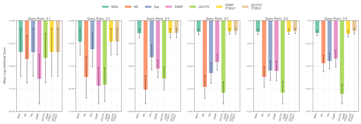
This figure presents the mean log-likelihood scores and their standard deviations for different methods (MAX, ML, Seq, SSMP, GUIDE, SSMP+ITSELF, GUIDE+ITSELF) across various query ratios (0.1 to 0.9) for Probabilistic Circuits (PCs) on the Audio dataset. Each bar represents a different method, allowing for a comparison of their performance under different query conditions. Higher scores indicate better performance.

This figure presents a comparison of various methods for solving the Most Probable Explanation (MPE) task across different probabilistic models (PMs). The contingency tables illustrate the frequency with which one method outperforms another in terms of log-likelihood scores. The color-coding (blue for row method superiority, red for column method superiority, darker shades indicating more frequent wins) provides a visual representation of the comparative performance. Different subfigures represent different types of PMs: PCs (Probabilistic Circuits), NAMs (Neural Autoregressive Models), and PGMs (Probabilistic Graphical Models).
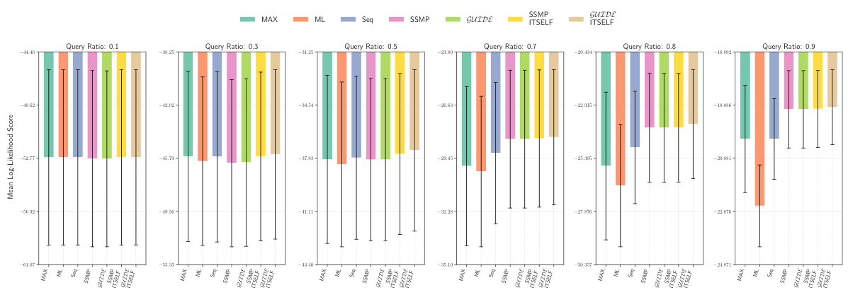
This figure displays the mean log-likelihood scores for different methods (MAX, ML, Seq, SSMP, GUIDE, SSMP+ITSELF, GUIDE+ITSELF) across various query ratios (0.1, 0.3, 0.5, 0.7, 0.8, 0.9) for PCs on the Audio dataset. Error bars represent the standard deviation. Higher scores suggest better performance.
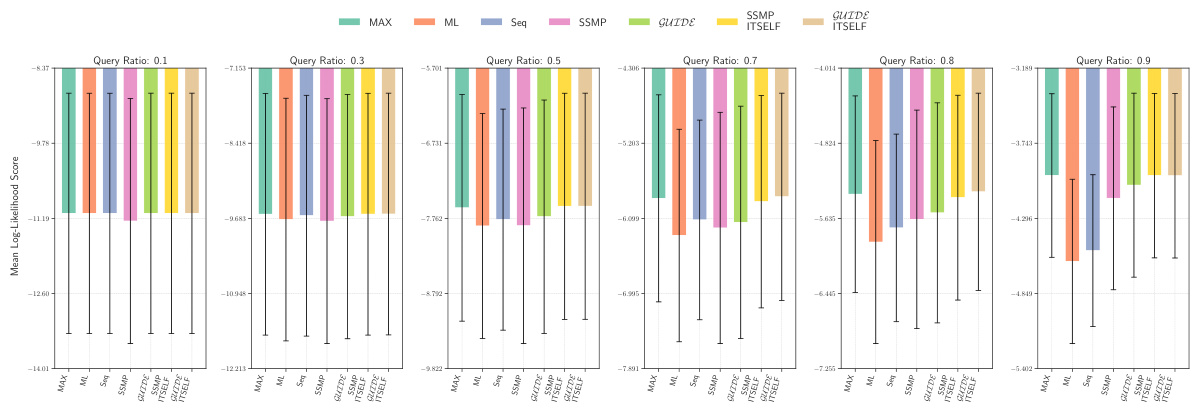
This figure displays the performance comparison of different MPE methods (MAX, ML, Seq, SSMP, GUIDE, SSMP+ITSELF, GUIDE+ITSELF) on the Audio dataset for PCs across various query ratios (0.1, 0.3, 0.5, 0.7, 0.8, 0.9). Each bar represents the average log-likelihood score for a given method and query ratio, with error bars indicating the standard deviation. Higher scores indicate better performance, showing the relative effectiveness of each method in maximizing the log-likelihood for different query sizes.
This figure presents the log-likelihood scores for different methods on the NLTCS dataset for Probabilistic Circuits (PCs). The methods compared are MAX, ML, Seq, SSMP, GUIDE, SSMP+ITSELF, and GUIDE+ITSELF. For each method, the scores are shown across various query ratios (0.1, 0.3, 0.5, 0.7, 0.8, and 0.9). Higher scores indicate better performance, suggesting the effectiveness of the proposed ITSELF and GUIDE approaches compared to the baseline methods.
This heatmap visualizes the inference times for MADE across different datasets and methods. Each cell represents the log of the inference time in microseconds. Lighter colors indicate faster inference times, highlighting the relative efficiency of different methods. The methods compared include traditional baselines (HC, SSMP, GUIDE) and the proposed methods with (ITSELF) and without (single forward pass) inference-time optimization. The different datasets used for the comparison are listed along the y-axis.
This figure displays the log-likelihood scores for different methods on the Audio dataset for Probabilistic Circuits (PCs). The methods compared are MAX, ML, Seq, SSMP, GUIDE, SSMP+ITSELF, and GUIDE+ITSELF. The scores are shown for different query ratios (0.1, 0.3, 0.5, 0.7, 0.8, 0.9). Higher scores indicate better performance. The figure helps in assessing the relative performance of different inference methods on a specific dataset and across varying query complexities.
This figure presents the log-likelihood scores for different methods (MAX, ML, Seq, SSMP, GUIDE, SSMP+ITSELF, GUIDE+ITSELF) on the NLTCS dataset for PCs across various query ratios. Each bar represents the mean log-likelihood score with error bars showing the standard deviation. Higher scores indicate better performance. This visualization helps compare the effectiveness of the proposed neural network approaches (SSMP, GUIDE, SSMP+ITSELF, GUIDE+ITSELF) with traditional polynomial-time baselines (MAX, ML, Seq) for PCs across varying query ratios. The results show the impact of ITSELF and GUIDE in improving log-likelihood scores compared to the baselines.
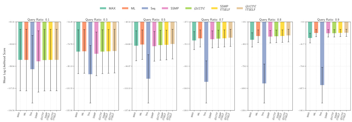
This figure displays the log-likelihood scores for the NLTCS dataset across different query ratios (0.5, 0.7, 0.8, and 0.9). Each bar represents the mean log-likelihood score for a given method (HC, SSMP, GUIDE, SSMP + ITSELF, and GUIDE + ITSELF), with error bars showing the standard deviation. Higher scores indicate better performance, demonstrating the effectiveness of ITSELF and GUIDE in improving the log-likelihood scores compared to baselines and other neural approaches.
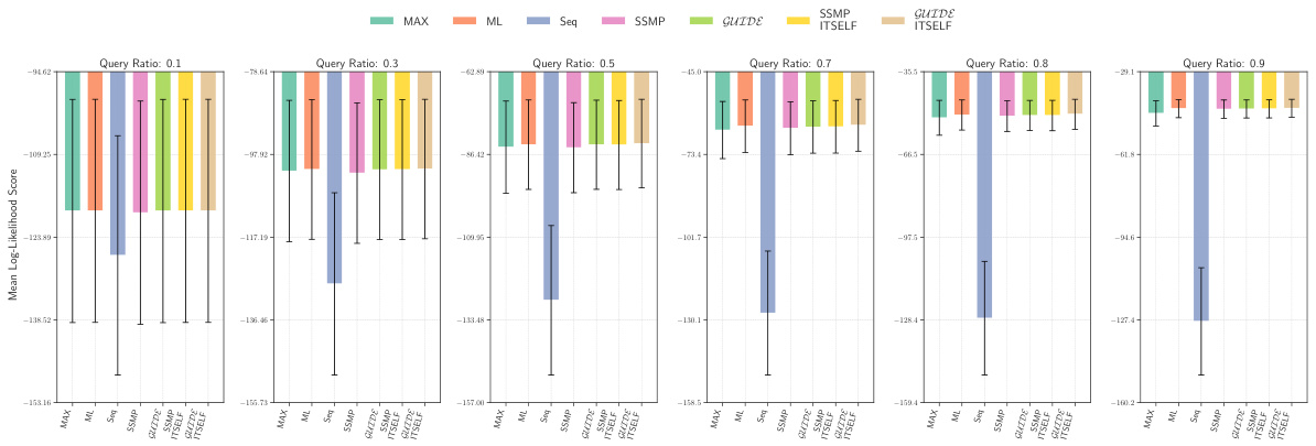
This figure displays the mean log-likelihood scores achieved by different methods (HC, SSMP, GUIDE, SSMP+ITSELF, GUIDE+ITSELF) on the NLTCS dataset for Neural Autoregressive Models (NAMs). The x-axis represents different query ratios (the proportion of variables included in the query), and the y-axis represents the mean log-likelihood score. Error bars indicate the standard deviation. Higher scores indicate better model performance.
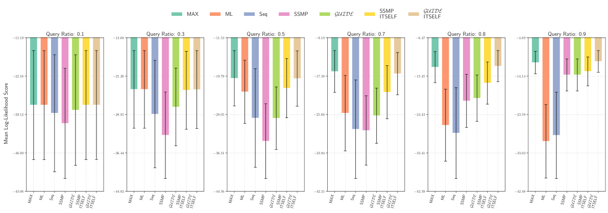
This figure presents two heatmaps visualizing the percentage difference in mean log-likelihood (LL) scores between the proposed method (GUIDE + ITSELF) and the MAX baseline. The top heatmap shows results for Probabilistic Circuits (PCs), while the bottom one illustrates results for Neural Autoregressive Models (NAMs). Each heatmap’s rows represent datasets, while columns depict varying query ratios. Green cells indicate superior performance of the proposed method over the baseline. Darker shades correspond to larger percentage differences.
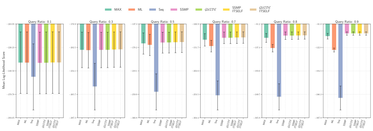
This figure presents two heatmaps visualizing the percentage difference in mean log-likelihood (LL) scores between the GUIDE+ITSELF method and the MAX baseline for Probabilistic Circuits (PCs) and Neural Autoregressive Models (NAMs). The y-axis represents datasets categorized by variable count, while the x-axis displays the query ratio. Green cells indicate that GUIDE+ITSELF outperforms MAX, with darker shades signifying a larger performance advantage. The top heatmap shows results for PCs, while the bottom shows results for NAMs. The figure highlights the superior performance of GUIDE+ITSELF, especially as problem complexity increases with larger query sets.
Full paper#
