↗ OpenReview ↗ NeurIPS Proc. ↗ Chat
TL;DR#
Bayesian persuasion studies how an informed sender influences a receiver’s actions by strategically releasing information. However, existing models unrealistically assume the sender knows either the receiver’s preferences or the prior probability distribution of different states, or both. This makes these models unsuitable for real-world applications where such information is often unavailable.
This research introduces a novel approach that eliminates this knowledge assumption. It presents a learning algorithm designed to minimize the sender’s regret (difference between the actual utility and the optimal utility) even without knowing the receiver or the prior. The algorithm learns the receiver’s best responses by cleverly searching a space of signalling schemes, enabling the sender to achieve sublinear regret (the regret grows sublinearly with the number of rounds). The authors also provide strong theoretical bounds, showing their algorithm’s regret guarantees are optimal.
Key Takeaways#
Why does it matter?#
This paper is crucial because it tackles a significant limitation in existing Bayesian persuasion models by removing the unrealistic assumption of sender knowledge about the receiver and the prior distribution. This opens new avenues for research in more realistic and practical applications, improving the applicability of Bayesian persuasion models in various fields and driving further development in online learning algorithms.
Visual Insights#

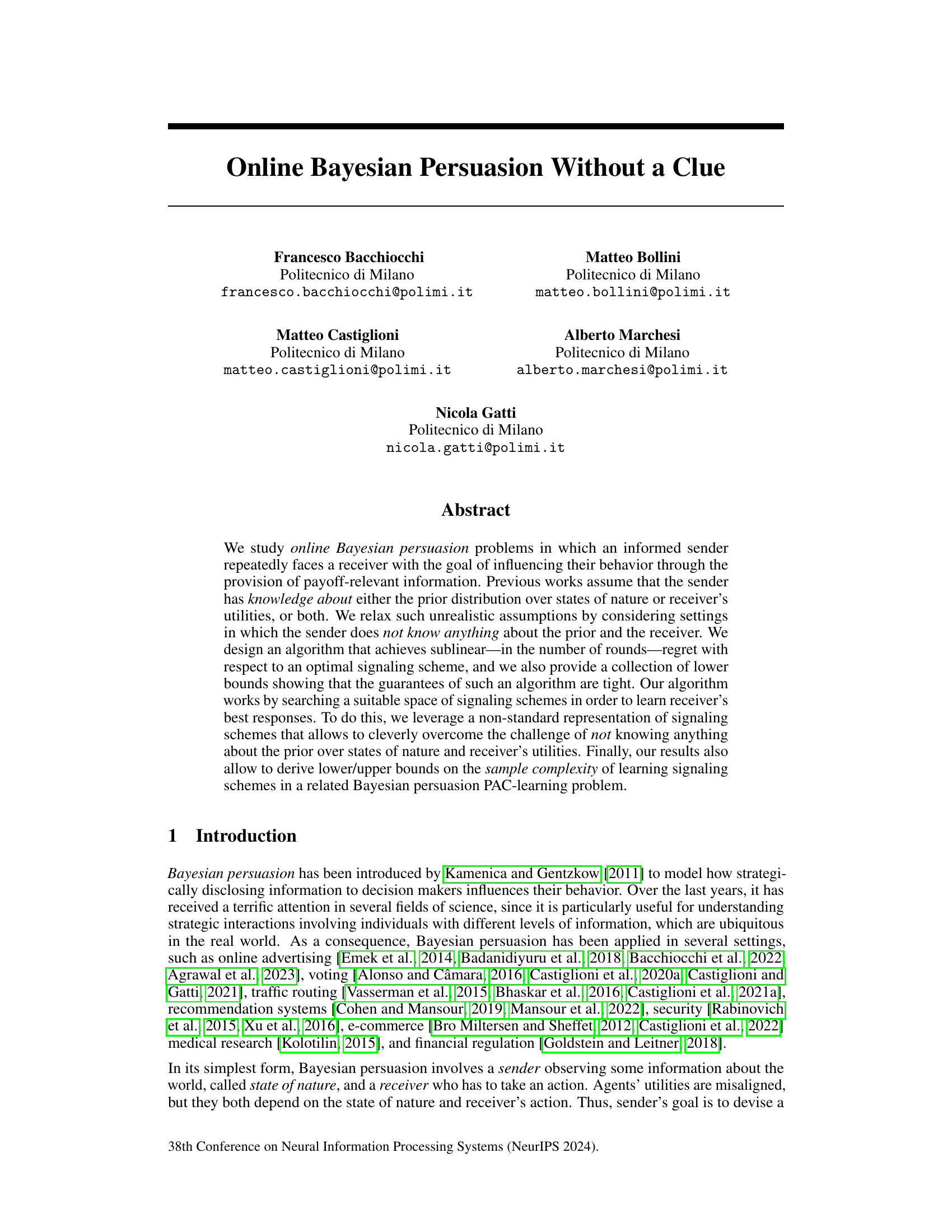
The figure shows a graphical representation of the sets X□(ai) and X△(ai) which are used to define the space of possible signaling schemes. The figure shows how the space of possible slices (X□) of signaling schemes is partitioned into regions based on the best-response action (a) for the receiver given that slice. Each region, denoted as X□(ai), represents the set of slices for which action ai is a best response. The figure also illustrates how the normalized slices (X△) are similarly partitioned.
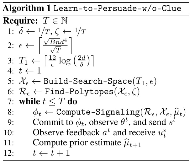
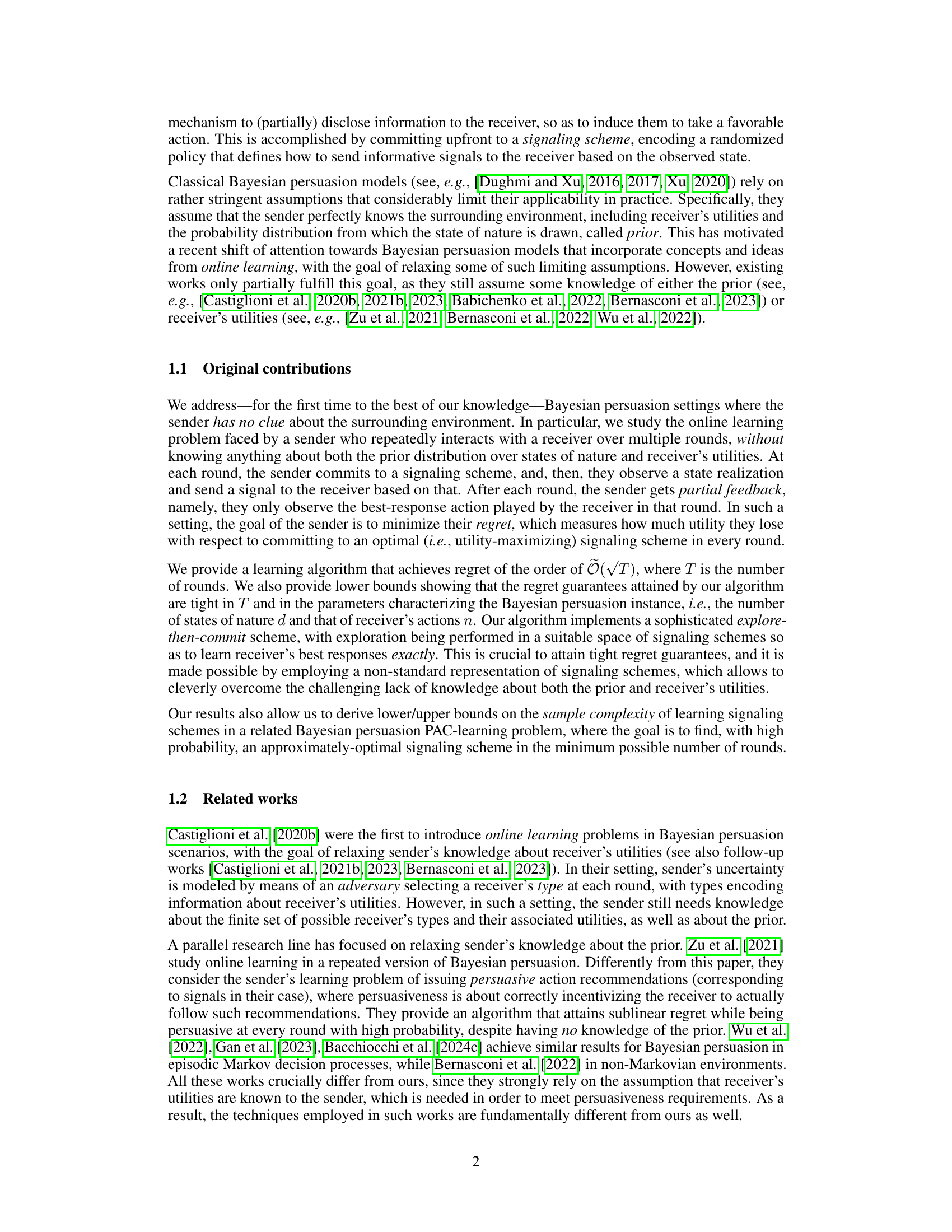
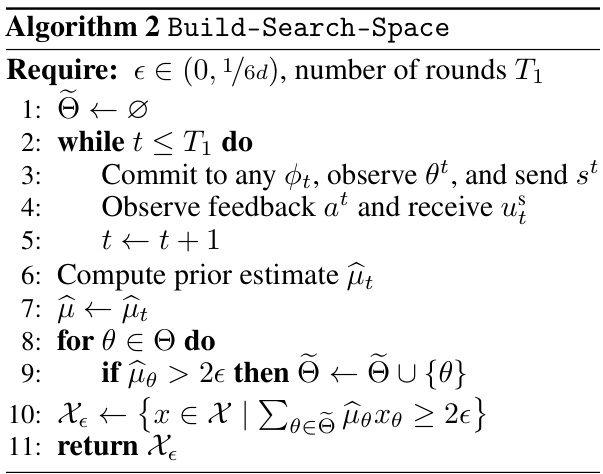
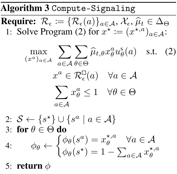
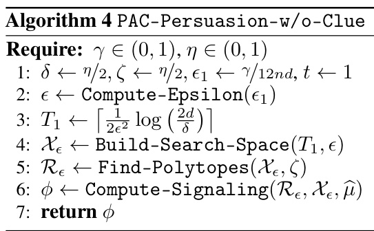
This algorithm addresses the online Bayesian persuasion problem where the sender has no prior knowledge about the receiver’s utilities or the prior distribution over states of nature. It uses a three-phase approach: building a search space of signaling schemes, finding the polytopes defined by receiver best responses, and computing approximately optimal signaling schemes. The algorithm achieves sublinear regret.
In-depth insights#
Prior-Free Persuasion#
Prior-free persuasion presents a significant advancement in Bayesian persuasion by removing the unrealistic assumption of the sender’s prior knowledge of the receiver’s utility or the prior distribution. This approach tackles the inherent challenge of strategic information disclosure in scenarios where the sender is uncertain about the receiver’s preferences and the underlying state of nature. Instead of relying on known priors, prior-free methods focus on learning receiver behavior through repeated interactions and feedback. This leads to algorithms that dynamically adapt their signaling strategies, converging towards near-optimal solutions. The core innovation involves cleverly navigating the space of possible signaling schemes to efficiently learn receiver best responses without prior assumptions. While computationally demanding in the general case, prior-free approaches are theoretically grounded and offer a more practical and robust solution to real-world Bayesian persuasion problems.
Regret Bounds#
Analyzing regret bounds in online Bayesian persuasion is crucial for evaluating algorithm performance. Tight bounds demonstrate the optimality of the proposed algorithms, indicating that no significant improvement is possible without altering underlying assumptions. Sublinear regret bounds, such as O(√T), suggest efficient learning, where the regret grows slower than the number of rounds. However, the specific form of the bounds often depends on problem parameters like the number of states or actions, implying that computational complexity can vary considerably depending on these factors. The presence of exponential dependencies in the bounds highlights computational challenges in high-dimensional problems. Comparing upper and lower regret bounds provides a complete picture of algorithm effectiveness, helping to establish the algorithm’s limitations and potential for future enhancements. The focus on both upper and lower bounds is essential for a rigorous analysis. Finally, investigating sample complexity bounds sheds light on the data requirements for achieving desired levels of accuracy.
Slice Representation#
The concept of ‘Slice Representation’ in a Bayesian persuasion setting appears crucial for handling scenarios where the sender lacks prior knowledge of the receiver’s utilities and the state of nature’s distribution. This representation cleverly focuses on the signal-specific components of the signaling scheme, abstracting away the sender’s uncertainty about the overall distribution. By representing a signaling scheme as a set of slices, each corresponding to a single signal, the algorithm effectively learns the receiver’s best responses without directly estimating the prior or utility function. This approach dramatically simplifies the learning process by reducing the dimensionality of the search space. Learning happens in the space of slices, enabling the algorithm to overcome the challenges posed by unknown parameters, hence achieving sublinear regret. The cleverness lies in recognizing that the receiver’s actions depend only on the slice’s attributes, not the entire signaling scheme. This is a significant innovation in online Bayesian persuasion, as it relaxes the stringent knowledge assumptions of prior works.
PAC Learning#
PAC (Probably Approximately Correct) learning offers a theoretical framework for analyzing machine learning algorithms. It focuses on the probability that a learned hypothesis will generalize well to unseen data, a crucial aspect often overlooked in simpler analyses. In the context of Bayesian persuasion, PAC learning could be applied to assess how quickly and reliably a sender can learn an effective signaling strategy given limited interactions and uncertain information about the receiver’s preferences and the state of nature. A key challenge in applying PAC learning to this setting lies in defining what constitutes a ‘correct’ or ‘approximately correct’ signaling scheme, given the inherent stochasticity of Bayesian games. Successfully framing the problem in a PAC learning context would provide strong guarantees on the sample complexity, i.e., the number of interactions required to achieve a desired level of accuracy in learning the optimal signaling strategy. The approach to applying PAC learning could involve carefully selected metrics that capture the sender’s performance, and rigorous analysis demonstrating that, with high probability, the learned strategy is within a specified tolerance of the optimal one.
Algorithm Analysis#
An Algorithm Analysis section for a Bayesian persuasion paper would delve into the time and space complexity of the proposed learning algorithm. It should rigorously establish upper and lower bounds on the algorithm’s regret or sample complexity, demonstrating its efficiency. Crucial to the analysis is discussing the dependence of these bounds on key parameters like the number of states of nature, actions, and rounds. Proofs of the theoretical results are vital, and the analysis should address the algorithm’s scalability to larger problem instances. A robust analysis also considers the impact of imperfect feedback on the algorithm’s performance. Finally, the analysis should compare the algorithm’s efficiency with existing solutions, potentially highlighting its advantages and limitations in various settings.
More visual insights#
More on tables
This table visually represents the sets Xº(ai) and X△(ai) which are crucial in the paper’s proposed algorithm for Bayesian persuasion. Xº(ai) represents the set of unnormalized slices (d-dimensional vectors) where action ai is a best response for the receiver, and X△(ai) is the normalized version of Xº(ai). The table helps illustrate how these sets form a covering of the space of possible slices and the relationship between them, which is essential to the learning process in the algorithm.
This table visually represents the sets X (ai) and X△(ai) for a Bayesian persuasion instance with two states of nature and three receiver actions. The sets represent regions in a two-dimensional space, where each region corresponds to a receiver’s best response action (a1, a2, or a3) to the sender’s signal. The figure aids in visualizing how the algorithm in the paper learns to partition the signal space based on these regions. The x-axis and y-axis represent the probabilities of the sender’s signals relating to the different states of nature.
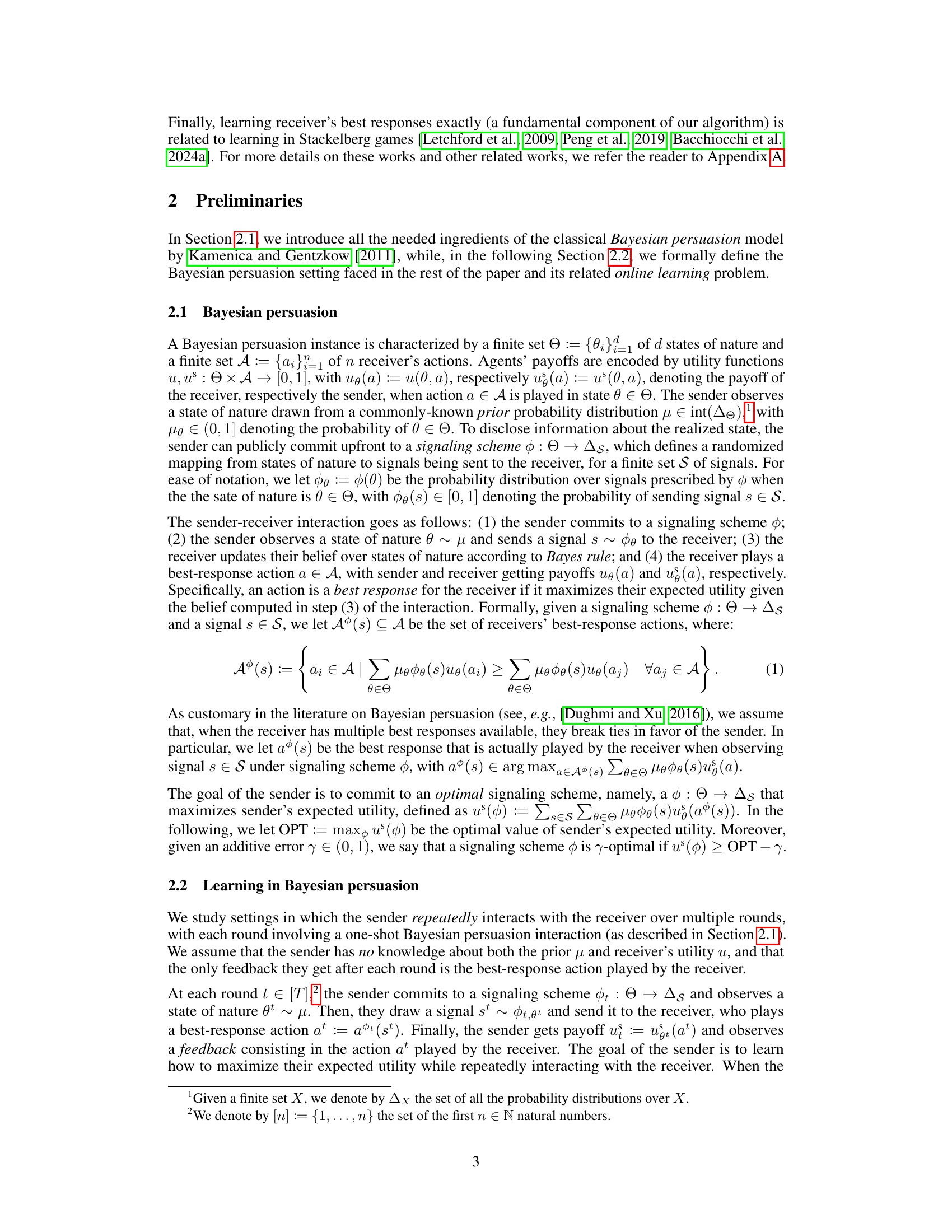
The table shows the upper and lower bounds on the regret, which measures how much the sender loses in terms of utility compared to an optimal signaling scheme in each round. The regret is shown as a function of the number of rounds (T), the number of states of nature (d), and the number of receiver actions (n). The upper bound is achieved by the algorithm described in the paper, while the lower bounds indicate the tightness of the algorithm’s guarantees. These results are discussed further in Section 5 of the paper.

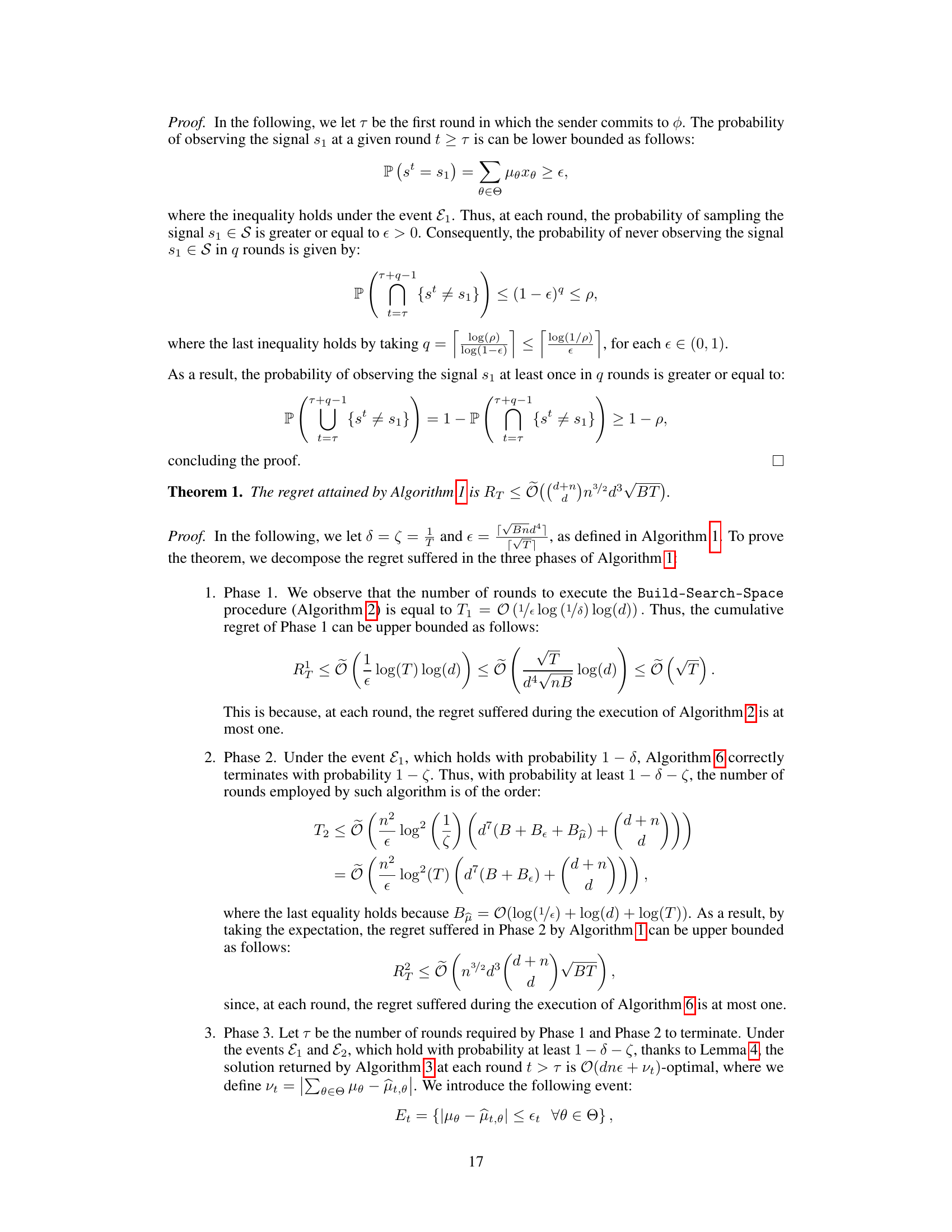
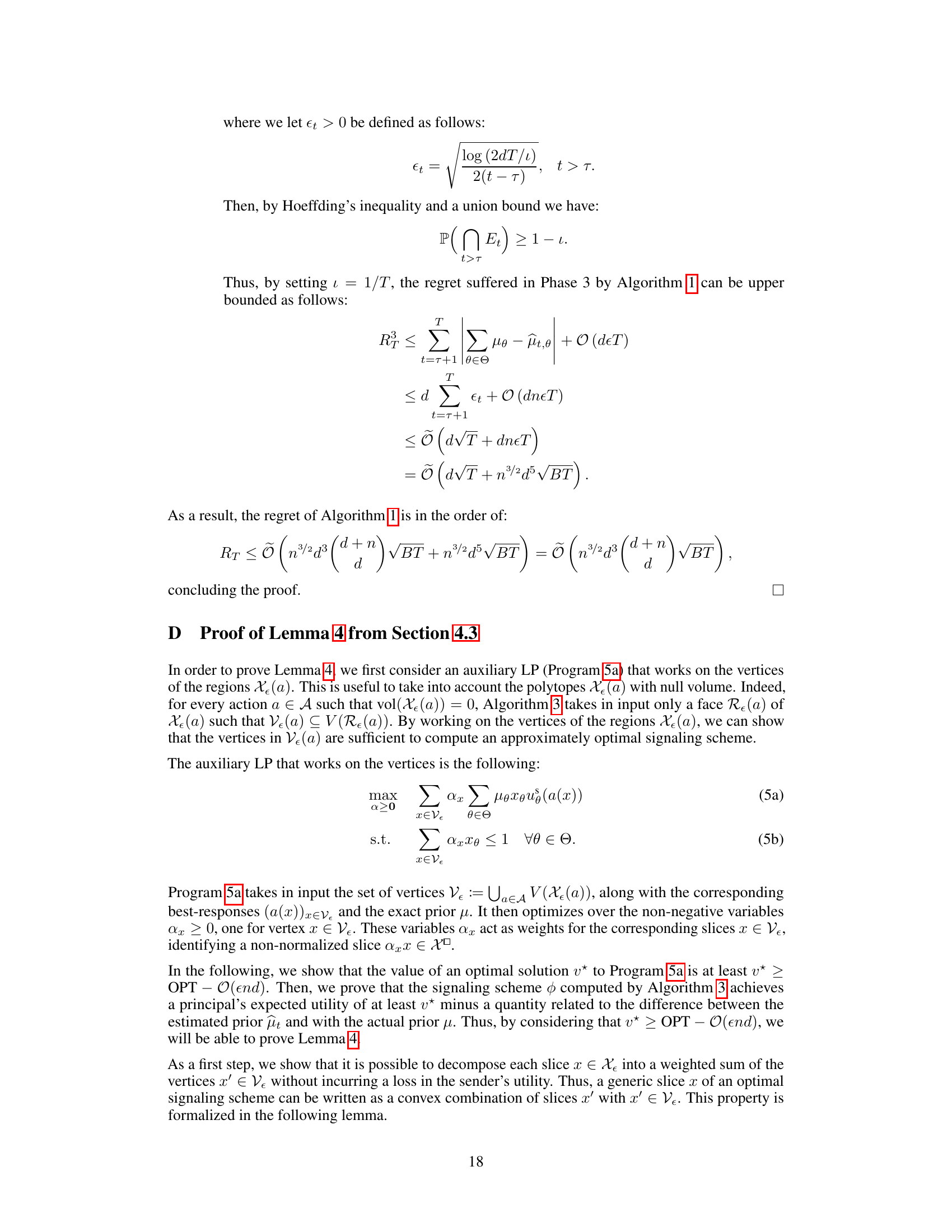
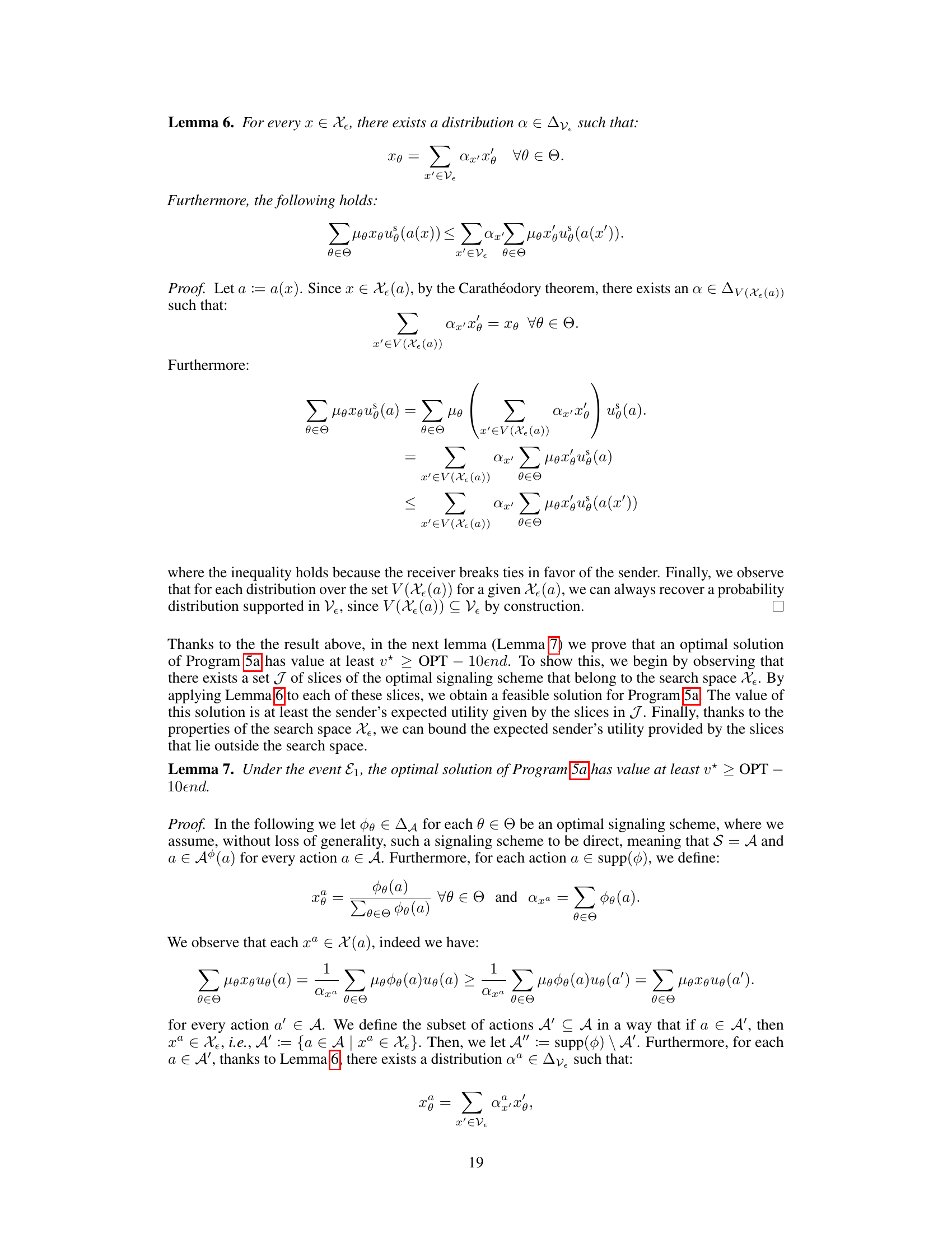
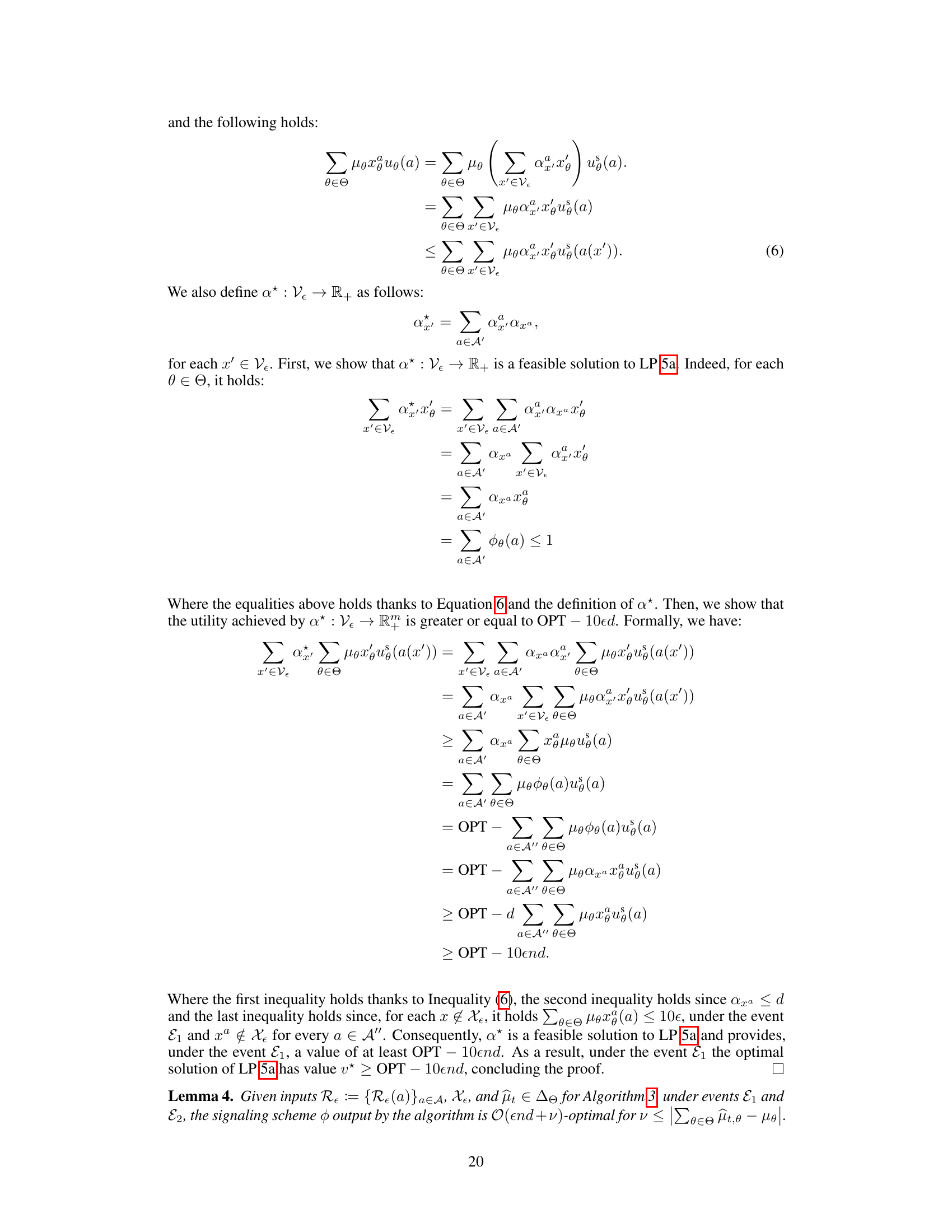
Algorithm 6 Find-Polytopes shows the pseudocode of the Find-Polytopes procedure. This procedure takes a search space of normalized slices (Xε) and a parameter ζ as input. It first calls the Find-Fully-Dimensional-Regions procedure to identify polytopes with volume greater than zero and their corresponding actions. Then, for actions not included in that set, it calls the Find-Face procedure to find a face of a polytope containing the vertices of interest. Finally, it returns a collection of polytopes, one for each action.
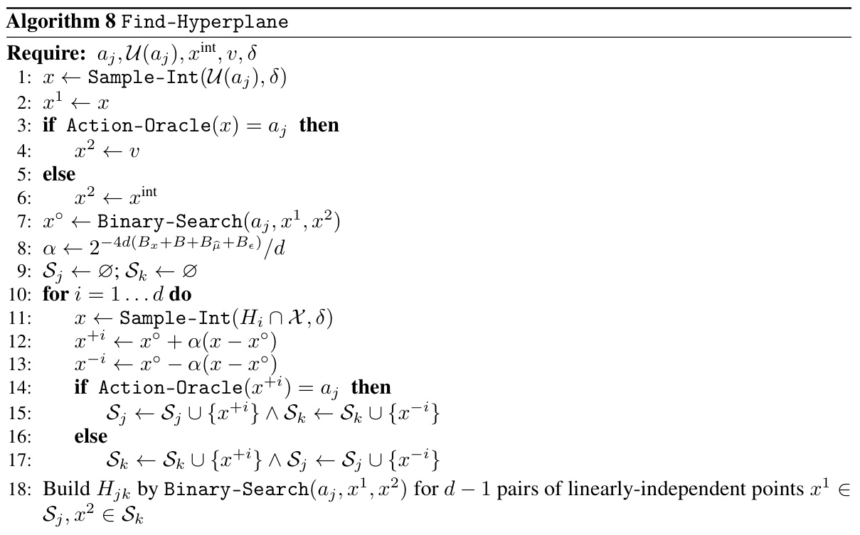
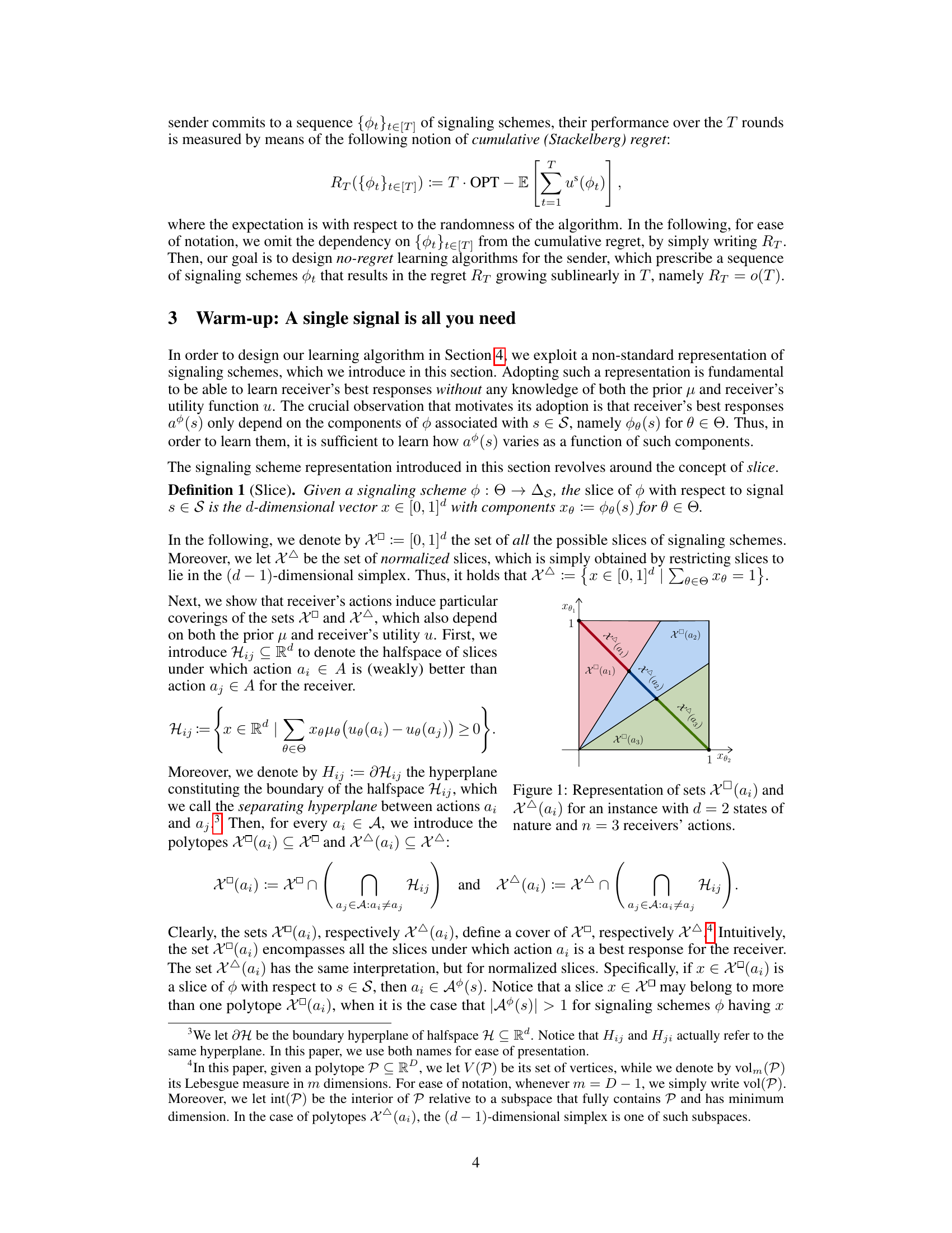
This table summarizes the key aspects of existing research in online Bayesian persuasion, highlighting the knowledge assumptions made by each work regarding the sender’s knowledge of the prior distribution over states of nature and/or the receiver’s utility function. It differentiates the approaches based on whether they relax assumptions about the prior, receiver utilities, or both, and whether the regret guarantees are tight.
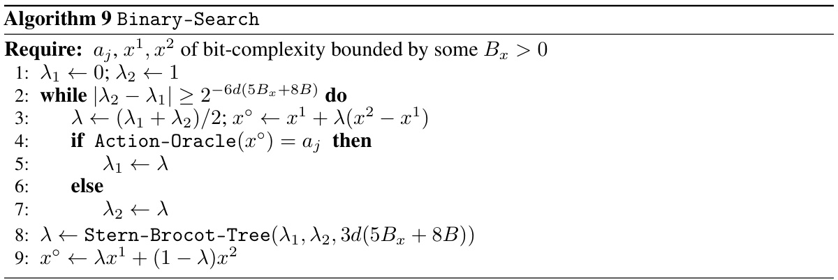
This table visually represents the sets X(ai) and X△(ai) which are crucial in understanding the algorithm. X(ai) and X△(ai) represent the sets of slices where action ai is a best response for the receiver in the unnormalized and normalized space respectively. The figure helps visualize how receiver’s actions induce particular coverings of the sets of slices, which are key to the proposed algorithm.

This algorithm samples a normalized slice from the interior of a given polytope. It takes as input a polytope P, where vold-1(P) > 0, and a parameter δ. The algorithm returns a normalized slice x ∈ int(P) satisfying certain conditions on its bit-complexity and the probability that it belongs to a given hyperplane. The algorithm first computes a normalized slice x0 as the average of d linearly-independent vertices of P. Then it samples a vector y from a suitable grid in the (d-1)-dimensional hypercube, scales it by a parameter ρ, and adds it to x0 to obtain x.
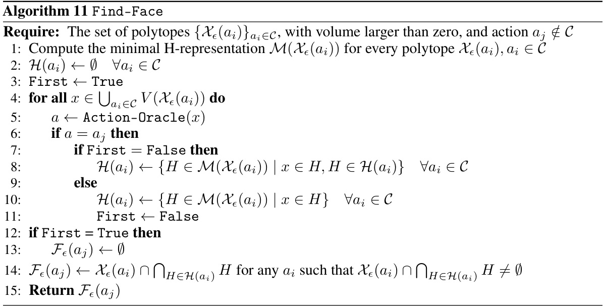
This table summarizes the notations used in the paper, including symbols for states of nature, actions, signals, probability distributions, and other mathematical concepts used in the Bayesian persuasion model.

This table shows the representation of sets X(ai) and X△(ai) with d=2 states of nature and n=3 receivers’ actions. It visually represents the polytopes formed by the intersection of halfspaces that define regions where a specific receiver’s action is optimal.
Full paper#
