↗ OpenReview ↗ NeurIPS Proc. ↗ Hugging Face ↗ Chat
TL;DR#
Prior research proposed scaling laws for optimal language model training, predicting the best model size given a compute budget. However, these laws produced conflicting predictions. This paper investigates the reasons for these discrepancies.
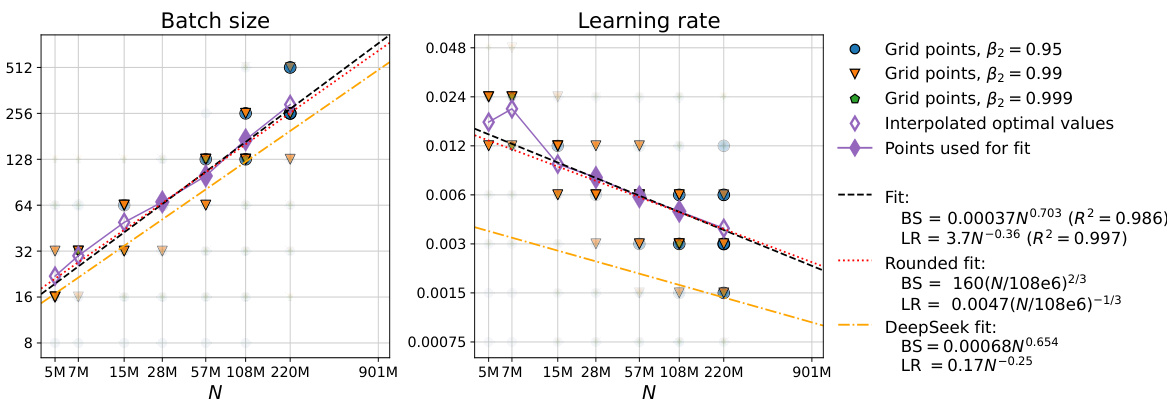
The study found three factors contributing to the differences: inaccurate accounting for last-layer computational cost, inappropriate warmup duration, and inconsistent optimizer tuning across different scales. By correcting these, the researchers achieved close agreement with an alternative scaling law (‘Chinchilla’) and demonstrated that learning rate decay wasn’t crucial for optimal scaling. Furthermore, they derived new scaling laws for learning rate and batch size, highlighting the importance of AdamW B2 parameter tuning at smaller batch sizes.
Key Takeaways#
Why does it matter?#
This paper is crucial because it resolves discrepancies in existing compute-optimal scaling laws for language models, offering a more accurate and reliable framework for resource allocation in large language model training. This directly impacts future model development, allowing for better performance with the same resources or achieving equivalent performance with reduced costs.
Visual Insights#
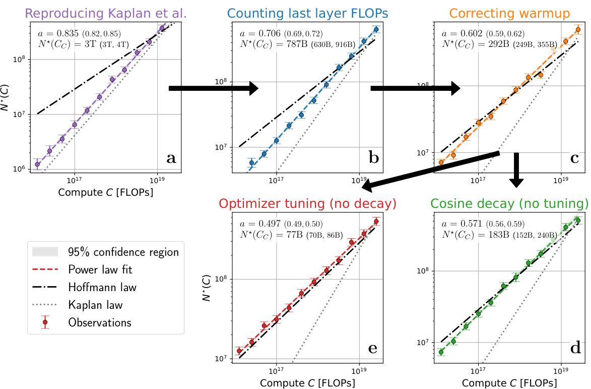
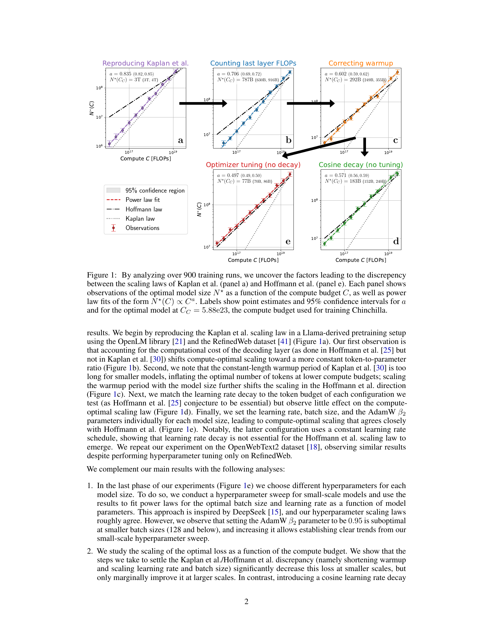
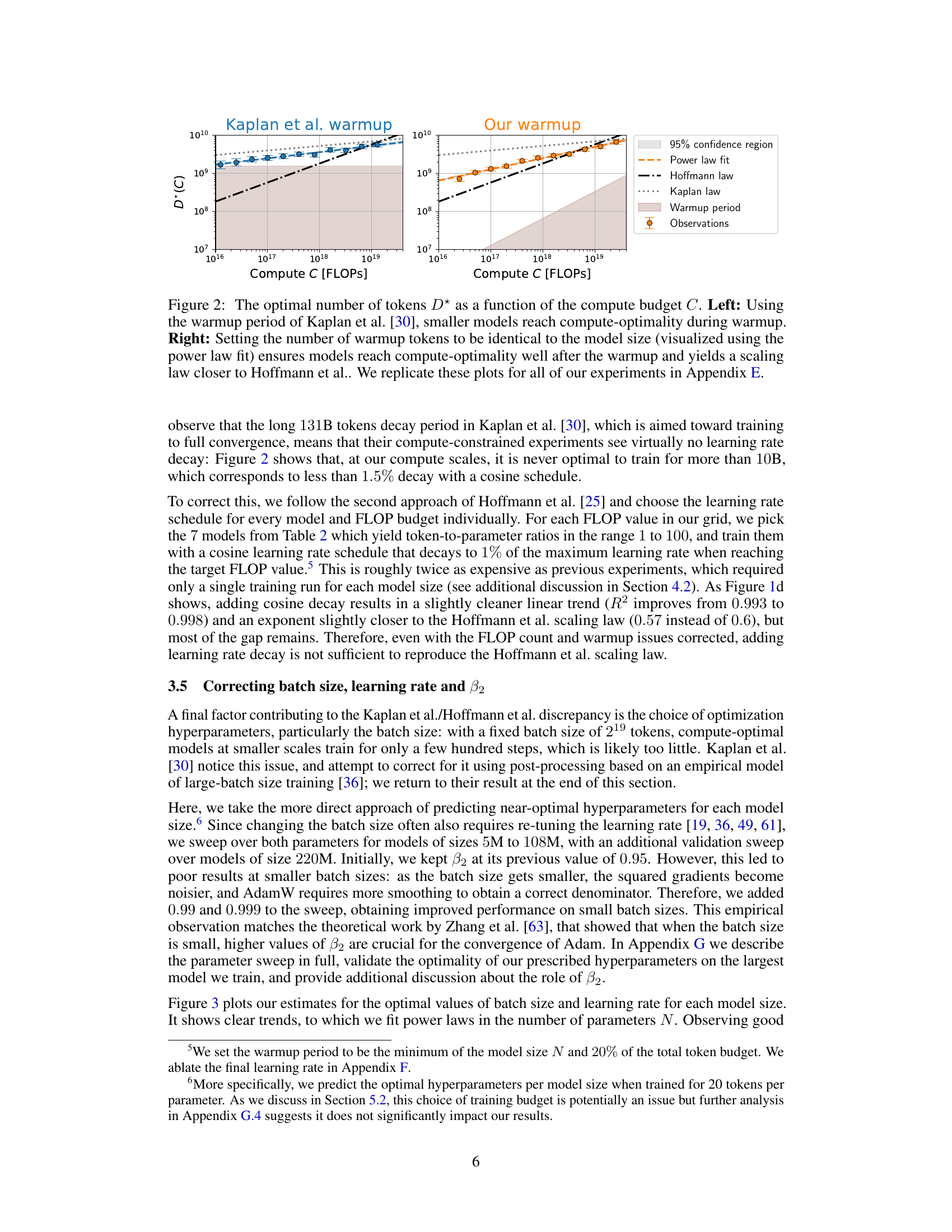
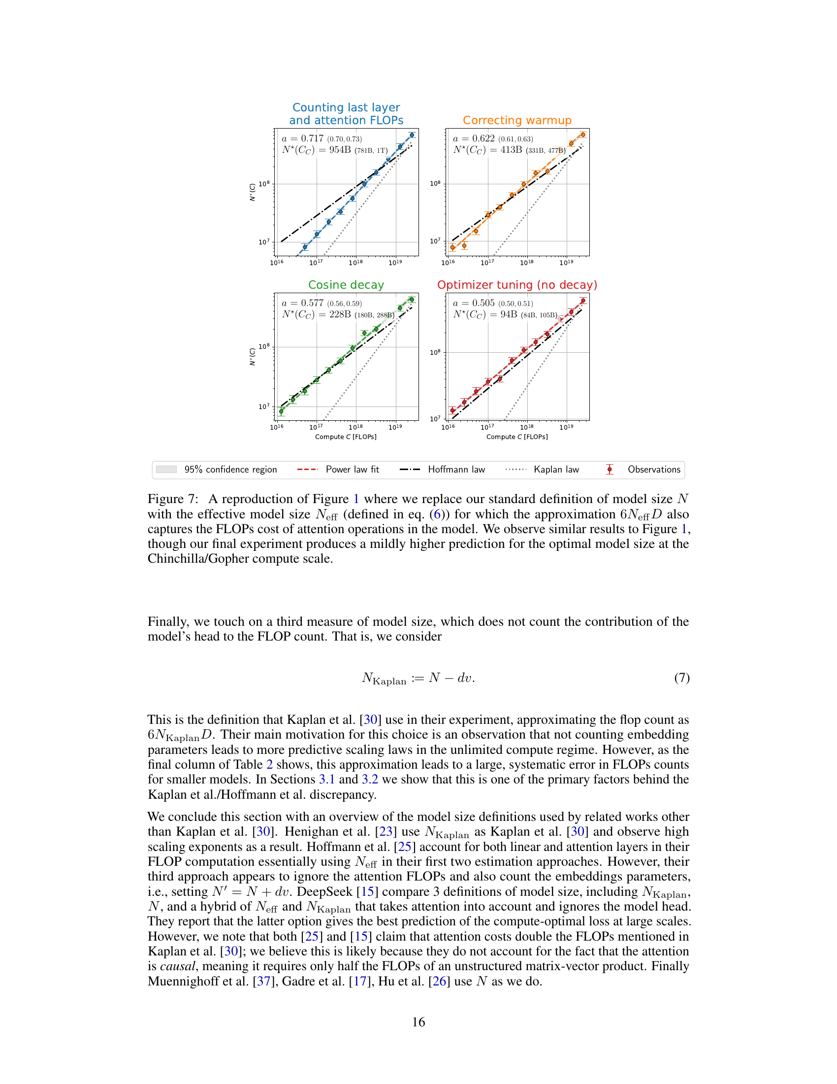
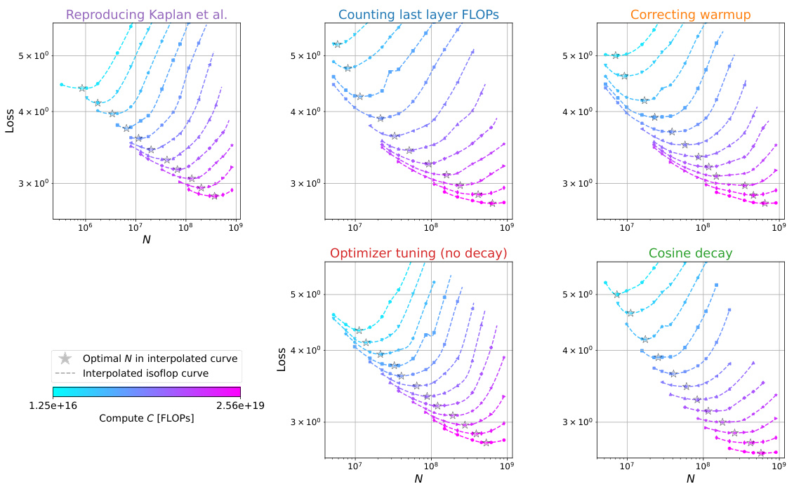
This figure shows the analysis of over 900 training runs to understand the discrepancies between the scaling laws proposed by Kaplan et al. and Hoffmann et al. It systematically investigates the impact of three factors: last layer computational cost, warmup duration, and optimizer tuning, on the optimal model size (N*) as a function of compute budget (C). Each panel represents a step in the analysis, starting with reproducing Kaplan et al.’s results and progressively correcting for the identified factors, ultimately demonstrating excellent agreement with Hoffmann et al.’s Chinchilla scaling law. The figure clearly visualizes the shift in the scaling law exponent (a) and optimal model size with each correction.
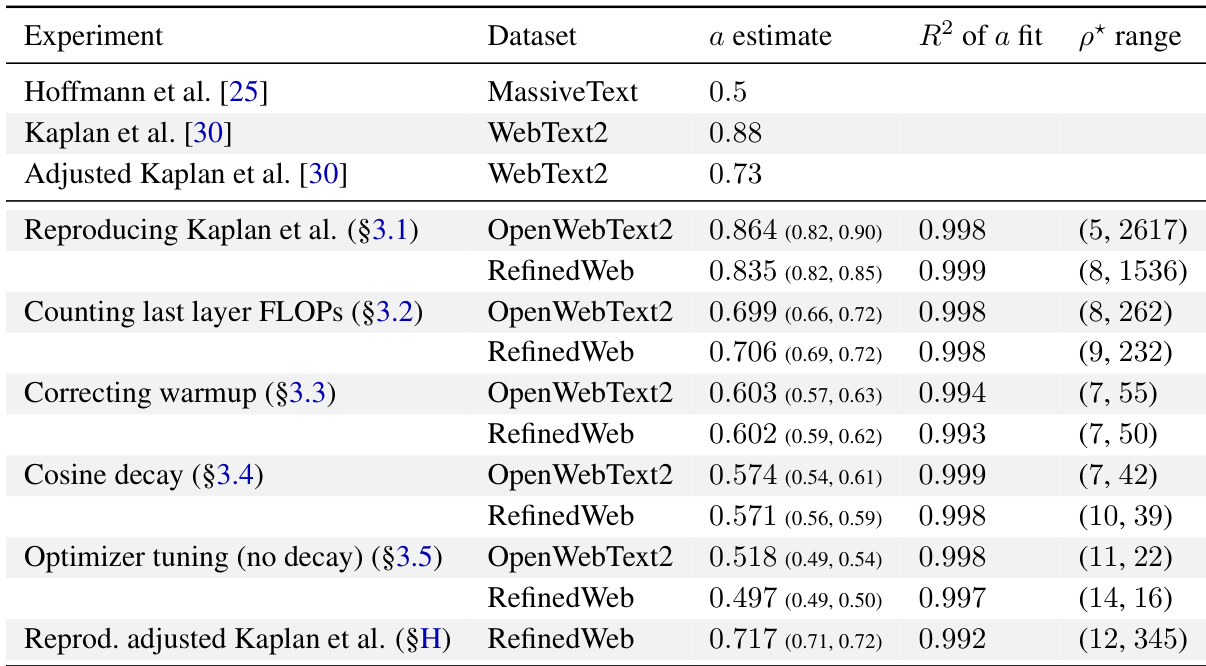
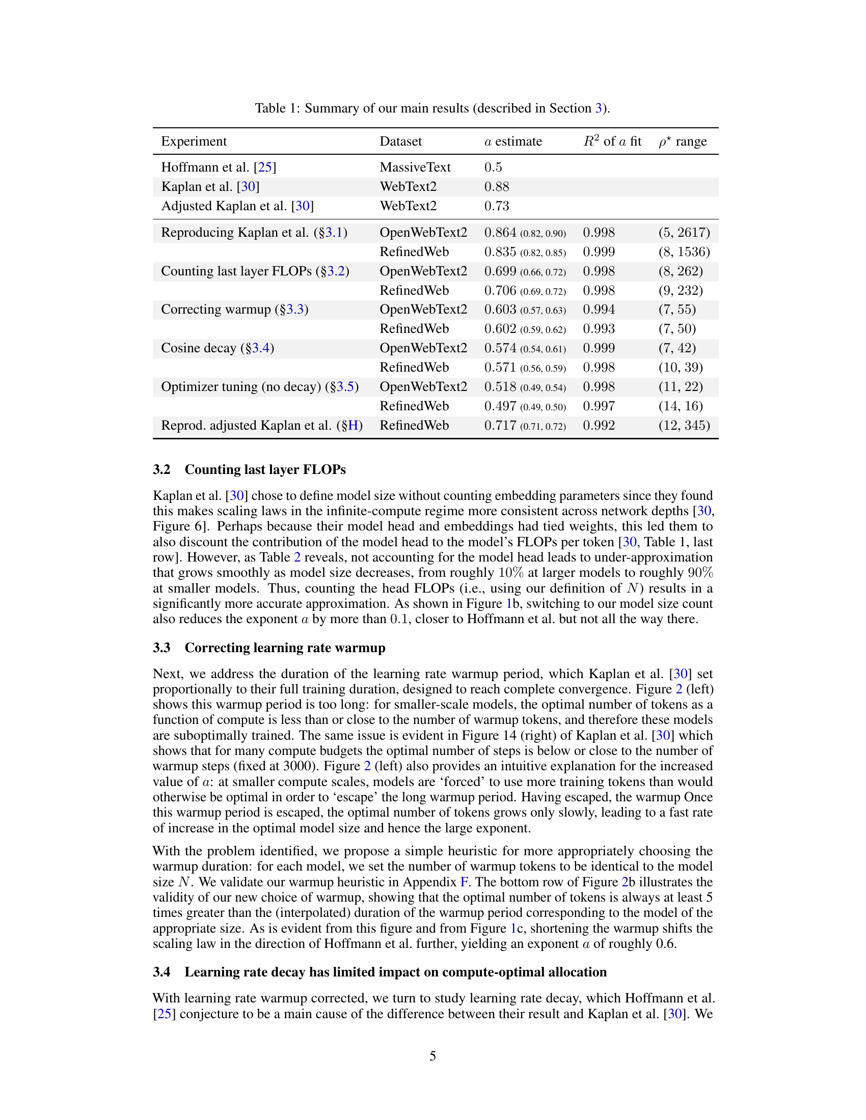
This table summarizes the key findings of the paper regarding compute-optimal scaling laws for large language models. It compares the scaling law exponent (a) obtained in this research with those reported by Hoffmann et al. [25] and Kaplan et al. [30], across different experiments and datasets. The R² values indicate the goodness of fit for the power-law models, and the p* range shows the span of optimal token-to-parameter ratios observed.
In-depth insights#
Scaling Discrepancies#
The paper investigates discrepancies in compute-optimal scaling laws for large language models, specifically addressing the conflict between the findings of Kaplan et al. and Hoffmann et al. The core of the discrepancy lies in differing assumptions and methodologies regarding computational cost calculations, particularly concerning the last layer’s FLOPs and the warmup phase of training. Inaccurate estimations of these factors significantly impact the predicted optimal model size and token-to-parameter ratio. The research systematically addresses these issues, highlighting the importance of precise FLOP accounting and appropriately scaled warmup durations. Furthermore, the study reveals that careful hyperparameter tuning, including AdamW B2 parameter optimization at smaller batch sizes, is crucial for achieving agreement with the Chinchilla scaling law. Ultimately, the work provides valuable insights into the nuances of model scaling, emphasizing that seemingly small methodological choices can have substantial consequences for the resulting scaling laws.
Optimal Hyperparams#
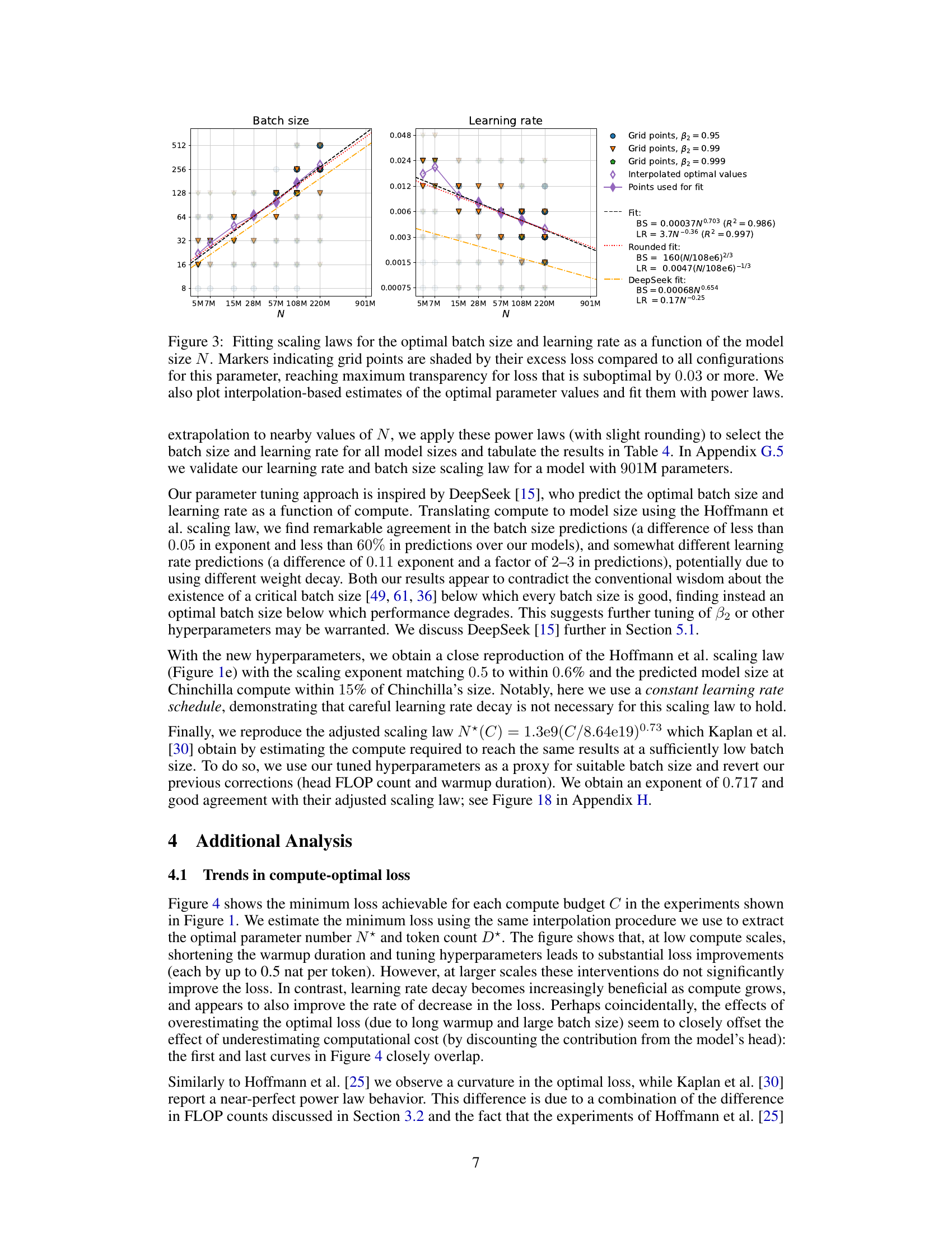
The optimal hyperparameter selection process is crucial for achieving peak performance in large language models. The paper delves into this, highlighting the interdependence of hyperparameters (learning rate, batch size, AdamW’s beta2) and their complex relationship with model size and compute budget. Finding optimal settings isn’t a one-size-fits-all approach; instead, scaling laws emerge which dictate how these parameters should change with increasing model size and compute. This necessitates a hyperparameter sweep for smaller models to establish optimal trends, which can then be extrapolated to larger models. Careful tuning of AdamW’s beta2 is particularly important at smaller batch sizes, significantly impacting performance. Simply employing a cosine learning rate decay, as suggested in prior work, is insufficient; constant learning rate schedules prove surprisingly effective. Ultimately, understanding these interactions allows for significant computational savings and better performance in training large language models.
Warmup & Decay#
The concepts of warmup and decay in the context of training large language models are crucial for optimization. Warmup gradually increases the learning rate from a small initial value, preventing drastic early updates that could hinder convergence. This is particularly important for large models and datasets. Decay, on the other hand, gradually decreases the learning rate as training progresses, to fine-tune the model after the initial large-scale adjustments of the warmup period. The optimal balance between warmup and decay is essential for achieving both efficient training and optimal model performance. The interplay between these two processes significantly impacts the compute-optimal scaling laws, affecting the model’s ability to converge to a solution efficiently. Different strategies for warmup and decay can lead to substantial variations in the optimal model size and token-to-parameter ratio. Mismatched or improperly designed schedules can result in suboptimal performance and slower convergence. Therefore, careful consideration and experimentation are required to establish the optimal strategies for specific model architectures, datasets, and training environments.
Compute-Optimal Loss#
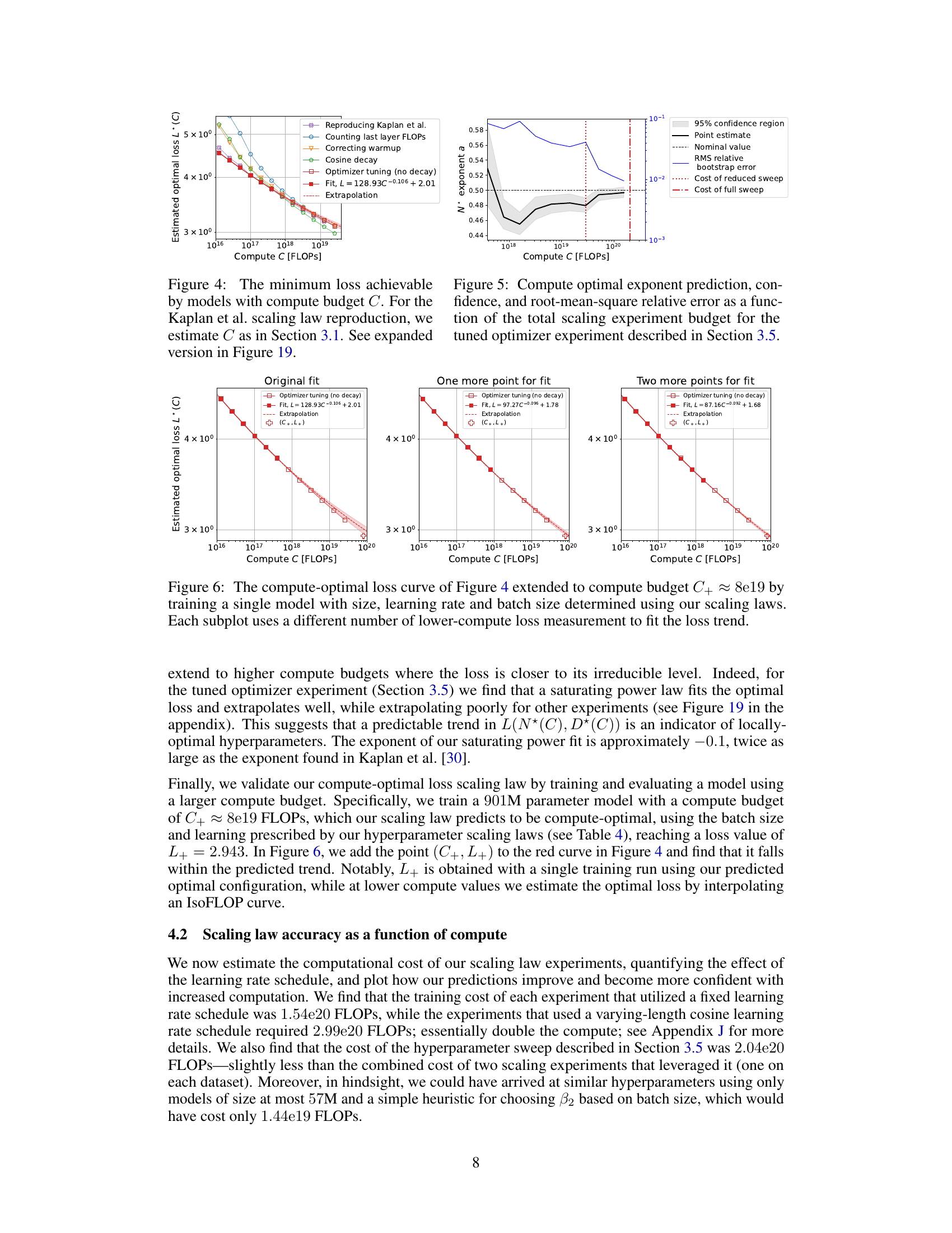
The concept of “Compute-Optimal Loss” in the context of large language model (LLM) training centers on finding the minimum loss achievable for a given compute budget. It’s a crucial aspect of scaling laws, aiming to optimize model performance within resource constraints. Analyzing the compute-optimal loss reveals insights into the efficiency of different training strategies and hyperparameter choices. A key finding is the trade-off between model size, dataset size, and the loss. While increasing compute generally reduces loss, the rate of improvement is not constant, suggesting diminishing returns. Further, carefully tuning hyperparameters like learning rate and batch size is essential for achieving near-optimal loss, underscoring that simply increasing model size isn’t the only path to improved performance. The analysis of compute-optimal loss thus provides valuable guidance in resource allocation for training LLMs, allowing researchers to maximize performance within defined budgetary limits.
Future Research#
Future research directions stemming from this work could explore several avenues. Extending the compute-optimal scaling laws to other modalities beyond language models (e.g., vision, audio) is crucial to establish the generality of these findings and understand modality-specific scaling behavior. Investigating the interaction between different hyperparameter tuning strategies and their effect on scaling laws would also be valuable, particularly exploring more sophisticated optimization methods and adaptive learning rate scheduling techniques. Further research could also focus on improving the accuracy of FLOP estimations, especially for complex architectures with a high degree of parallelism, to refine the precision of scaling law predictions. Finally, deeper analysis is needed to understand the reasons behind the observed loss curvature at larger scales and whether it reflects fundamental limitations or merely suboptimal hyperparameter choices. This would lead to a better understanding of the compute-optimal training paradigms and potential improvements to current training methodologies.
More visual insights#
More on figures

This figure displays a series of graphs illustrating how the authors of the paper investigated the discrepancies between two competing scaling laws for language models, those of Kaplan et al. and Hoffmann et al. Each panel shows the optimal model size (N*) plotted against compute budget (C), along with power law fits. The panels systematically show the effects of correcting different aspects of the training procedure, such as accounting for last layer computational cost, adjusting warmup duration, and considering scale-dependent optimizer tuning. The final panel demonstrates that, by addressing these factors, the authors obtain agreement with the Hoffmann et al. (‘Chinchilla’) scaling law, thereby explaining the previously observed discrepancy.
This figure presents a series of plots illustrating how different factors contribute to the discrepancy between the scaling laws proposed by Kaplan et al. and Hoffmann et al. for optimal language model scaling. Each subplot shows the optimal model size (N*) plotted against the compute budget (C), with power-law fits and confidence intervals. The subplots progressively correct three factors: last-layer computational cost, warmup duration, and scale-dependent optimizer tuning. The figure demonstrates that after correcting these three factors, the results align well with Hoffmann et al.’s Chinchilla scaling law.

This figure shows a series of plots that analyze the factors contributing to the discrepancy between the scaling laws proposed by Kaplan et al. and Hoffmann et al. for optimal language model scaling. Each subplot represents a step in the analysis, starting with a reproduction of Kaplan et al.’s results and progressively correcting for identified factors such as last layer computational cost, warmup duration, and optimizer tuning. The plots illustrate the optimal model size (N*) as a function of compute budget (C), showing how the corrected model aligns more closely with Hoffmann et al.’s findings.

This figure presents a series of plots visualizing the impact of various factors on the compute-optimal scaling of language models. It compares the scaling laws proposed by Kaplan et al. and Hoffmann et al., highlighting the discrepancies. Each subplot systematically isolates a contributing factor (e.g., last layer computational cost, warmup duration, optimizer tuning) by modifying the experimental setup and retraining models. The plots track the optimal model size (N*) against the compute budget (C), showcasing how each correction brings the experimental results closer to alignment with the Chinchilla scaling law.
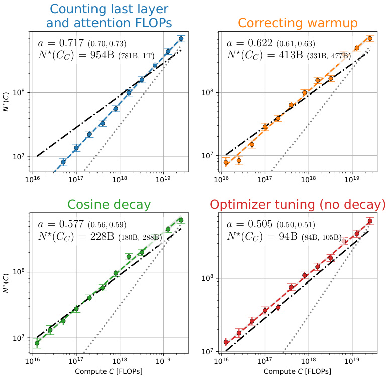
This figure shows the results of over 900 training runs to identify factors contributing to the discrepancy between the scaling laws proposed by Kaplan et al. and Hoffmann et al. Each subplot represents a step in the analysis, progressively correcting for factors like last layer computational cost, warmup duration, and optimizer tuning. The plots show optimal model size (N*) against compute budget (C) with power law fits. The final subplot shows excellent agreement with Hoffmann et al.’s Chinchilla scaling law after the corrections have been applied.
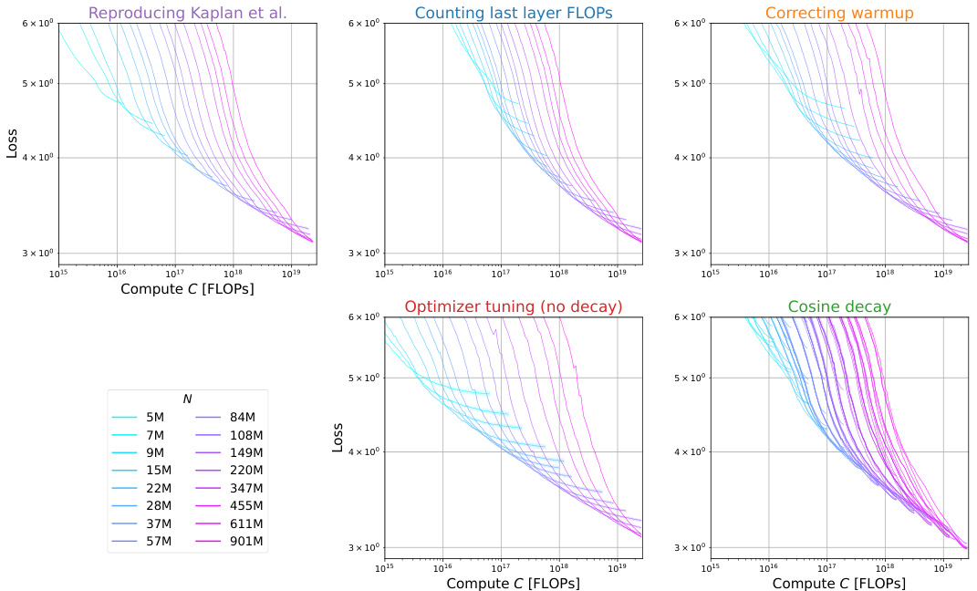
This figure presents a series of plots illustrating the effects of several factors on the compute-optimal scaling of language models, comparing the findings of Kaplan et al. and Hoffmann et al. It demonstrates how correcting for last layer computational cost, warmup duration, and optimizer tuning leads to a much closer agreement between the two scaling laws. The figure visually shows how adjusting for these three factors gradually shifts the observed scaling law from that of Kaplan et al. towards the Chinchilla scaling law proposed by Hoffmann et al.
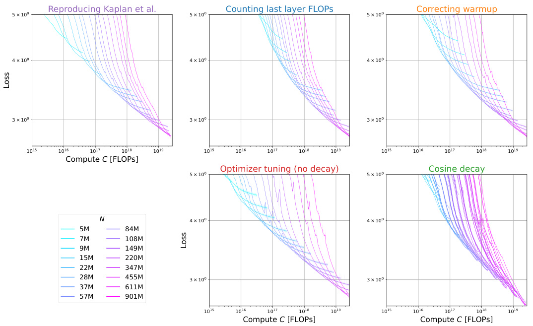
This figure presents a series of plots showing how the compute-optimal model size (N*) changes with compute budget (C) across different experimental settings. Each panel represents a different stage of refinement in the experimental setup: (a) Reproduces the original Kaplan et al. scaling law; (b) accounts for the computational cost of the last layer; (c) corrects the warmup duration; (d) uses a cosine learning rate decay without further tuning; (e) performs scale-dependent optimizer tuning, revealing a close match to the Chinchilla scaling law. The plots highlight how several factors, not initially accounted for, contribute to the discrepancy between the earlier Kaplan et al. and the later Chinchilla scaling laws.
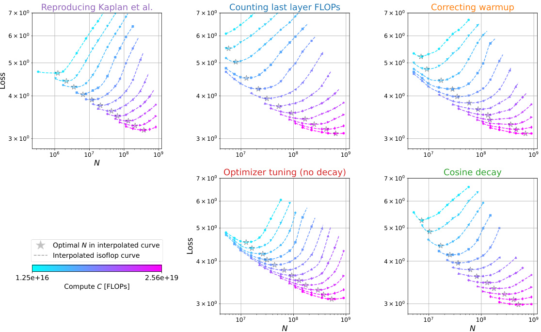
This figure shows a series of plots that analyze the discrepancies between the scaling laws proposed by Kaplan et al. and Hoffmann et al. for optimal language model size as a function of compute budget. By systematically reproducing Kaplan’s experiment and isolating specific factors (last layer computational cost, warmup duration, and optimizer tuning), the authors demonstrate how these factors contribute to the discrepancies. The plots visualize how correcting for these factors leads to a much closer agreement with Hoffmann et al.’s Chinchilla scaling law, ultimately disproving a hypothesis about learning rate decay put forth in the original Chinchilla paper.
This figure presents a series of plots illustrating the effects of various factors on the compute-optimal scaling of language models. The plots compare the scaling laws of Kaplan et al. and Hoffmann et al., highlighting the discrepancies and showing how those discrepancies can be resolved by addressing factors such as last layer computational cost, warmup duration, and optimizer tuning. Each plot shows the optimal model size (N*) as a function of compute budget (C), fitted to a power law of the form N*(C)∝C^a. The figure systematically corrects for each factor, revealing how the scaling law changes until it closely matches the Chinchilla scaling law.

This figure presents a series of graphs, each illustrating how modifications to the training process affect the optimal model size (N*) as a function of computational budget (C). It demonstrates how three key factors—last layer computational cost, warmup duration, and optimizer tuning—contribute to discrepancies between the scaling laws proposed by Kaplan et al. and Hoffmann et al. By systematically adjusting these factors, the authors demonstrate a pathway towards reconciliation of the two differing scaling laws.
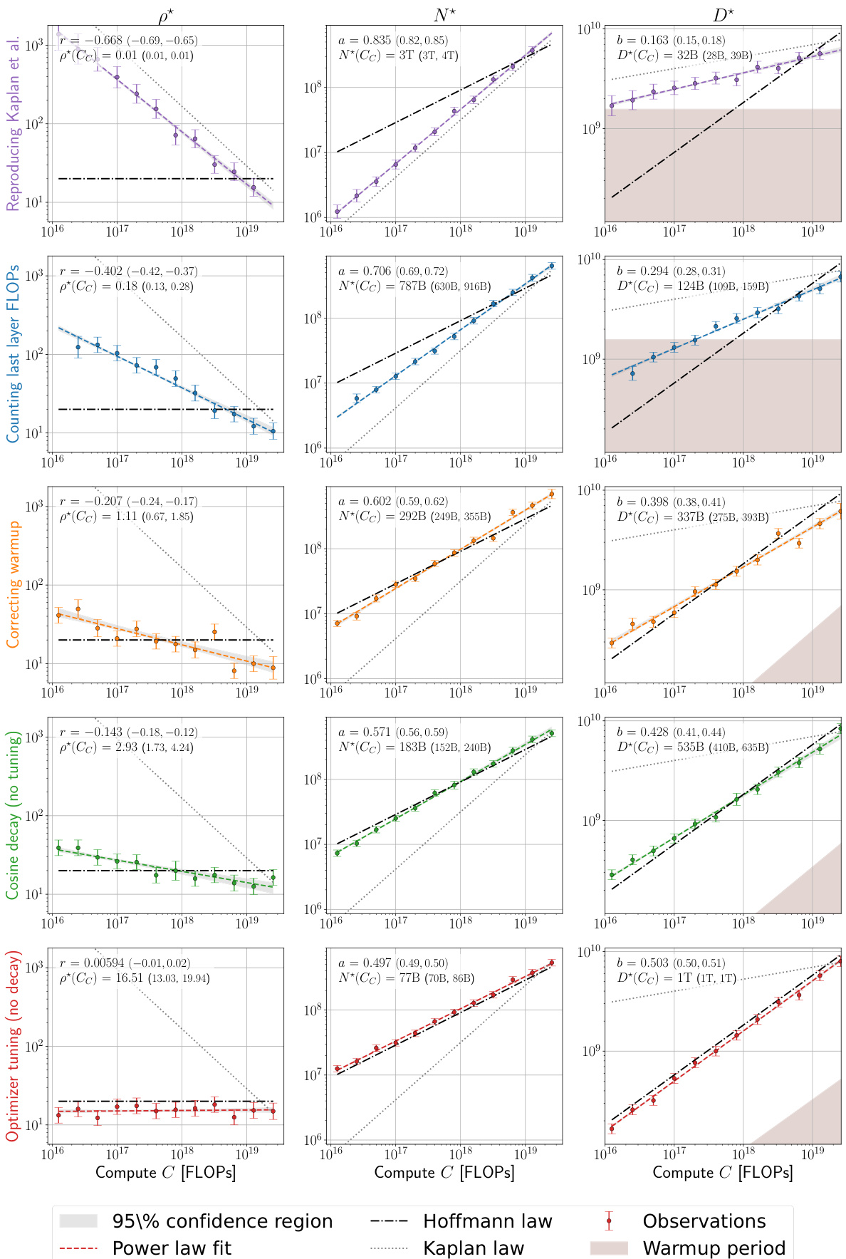
This figure presents a series of plots that investigate the discrepancies between the scaling laws proposed by Kaplan et al. and Hoffmann et al. for optimal language model training. The plots track the optimal model size (N*) against the compute budget (C) across various experimental setups. Each panel represents a different modification to the training process (e.g., accounting for last layer FLOPs, correcting warmup duration, or optimizer tuning). The goal is to isolate the factors that contribute to the differing predictions of the two scaling laws, ultimately demonstrating a close agreement with the Hoffmann et al. law after accounting for these factors.
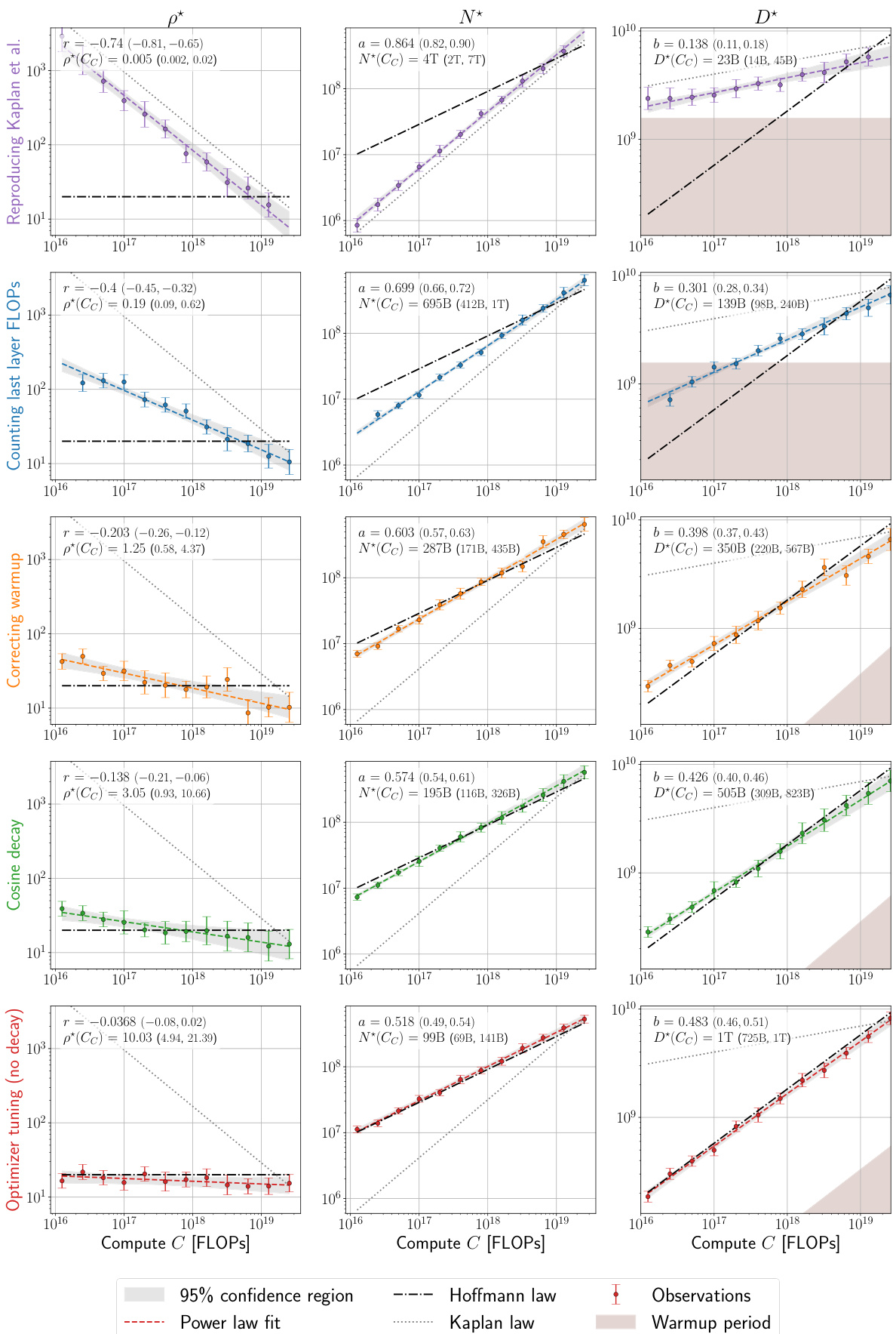
This figure presents a series of plots that investigate the discrepancies between the scaling laws proposed by Kaplan et al. and Hoffmann et al. for optimal language model training. Each subplot shows how the optimal model size (N*) changes with compute budget (C), with and without various corrections applied to address factors such as last layer computational cost, warmup duration, and optimizer tuning. By systematically correcting these factors, the figure demonstrates how the initially divergent scaling laws converge to a strong agreement, ultimately validating the findings of Hoffmann et al. The plots also provide 95% confidence intervals for the power-law exponent, offering a measure of uncertainty in the estimations.
This figure analyzes over 900 training runs to identify factors contributing to discrepancies between the scaling laws proposed by Kaplan et al. and Hoffmann et al. Each panel displays the optimal model size (N*) plotted against compute budget (C), along with power law fits. The figure demonstrates how various adjustments—including accounting for last layer FLOPs, correcting warmup, and optimizer tuning— progressively shift the Kaplan et al. scaling law towards agreement with the Hoffmann et al. (Chinchilla) scaling law.
This figure shows the results of an experiment to find the compute-optimal scaling law for large language models. It compares the scaling laws proposed by Kaplan et al. and Hoffmann et al., and systematically investigates three factors causing their discrepancy: the last layer’s computational cost, warmup duration, and scale-dependent optimizer tuning. Each subfigure displays how correcting each factor brings the results closer to agreement with Hoffmann et al.’s law. The experiment involved over 900 training runs.
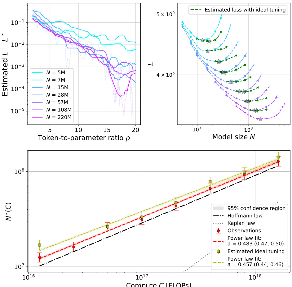
This figure shows a series of plots that analyze the factors contributing to the discrepancy between the scaling laws proposed by Kaplan et al. and Hoffmann et al. for optimal language model scaling. Each sub-plot represents a stage in the analysis, starting with a reproduction of Kaplan et al.’s results and progressively correcting for factors like last layer computational cost, warmup duration, and optimizer tuning. The final plot demonstrates excellent agreement with Hoffmann et al.’s Chinchilla scaling law. The plots illustrate how optimal model size (N*) changes as a function of compute budget (C), along with power law fits and confidence intervals to quantify the relationship.
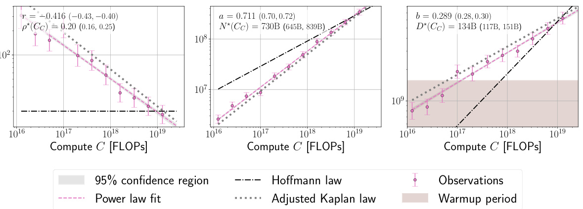
This figure shows the results of an experiment designed to investigate the discrepancies between the scaling laws of Kaplan et al. and Hoffmann et al. for optimal language model training. The experiment systematically varies three factors (last layer computational cost, warmup duration, and optimizer tuning) to understand their impact on the optimal model size (N*) as a function of compute budget (C). Each panel shows the results for a specific set of conditions, highlighting the progression of the relationship between N* and C as the factors are corrected. The final panel (e) shows good agreement with Hoffmann et al.’s Chinchilla scaling law, indicating the factors identified are key contributors to the discrepancy.
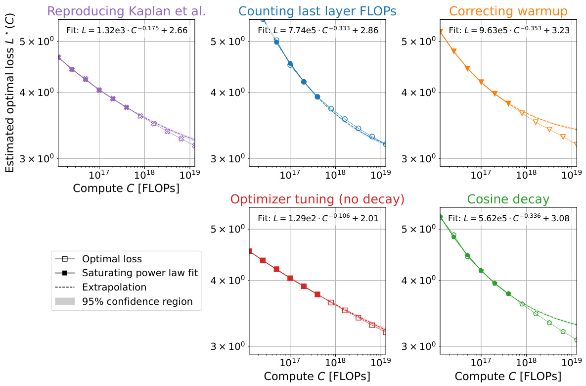
This figure presents a series of plots showing how the optimal model size (N*) scales with compute budget (C) under different experimental conditions. Starting with a reproduction of Kaplan et al.’s scaling law, the figure progressively refines the experiment to isolate and correct for factors contributing to the discrepancy between Kaplan et al.’s and Hoffmann et al.’s (Chinchilla) scaling laws. These factors include the computational cost of the last layer, warmup duration, and optimizer tuning. Each panel shows the observed data, a power-law fit, and the scaling laws from Kaplan et al. and Hoffmann et al. for comparison, highlighting the convergence towards agreement with Hoffmann et al.’s findings as the experimental conditions are refined.
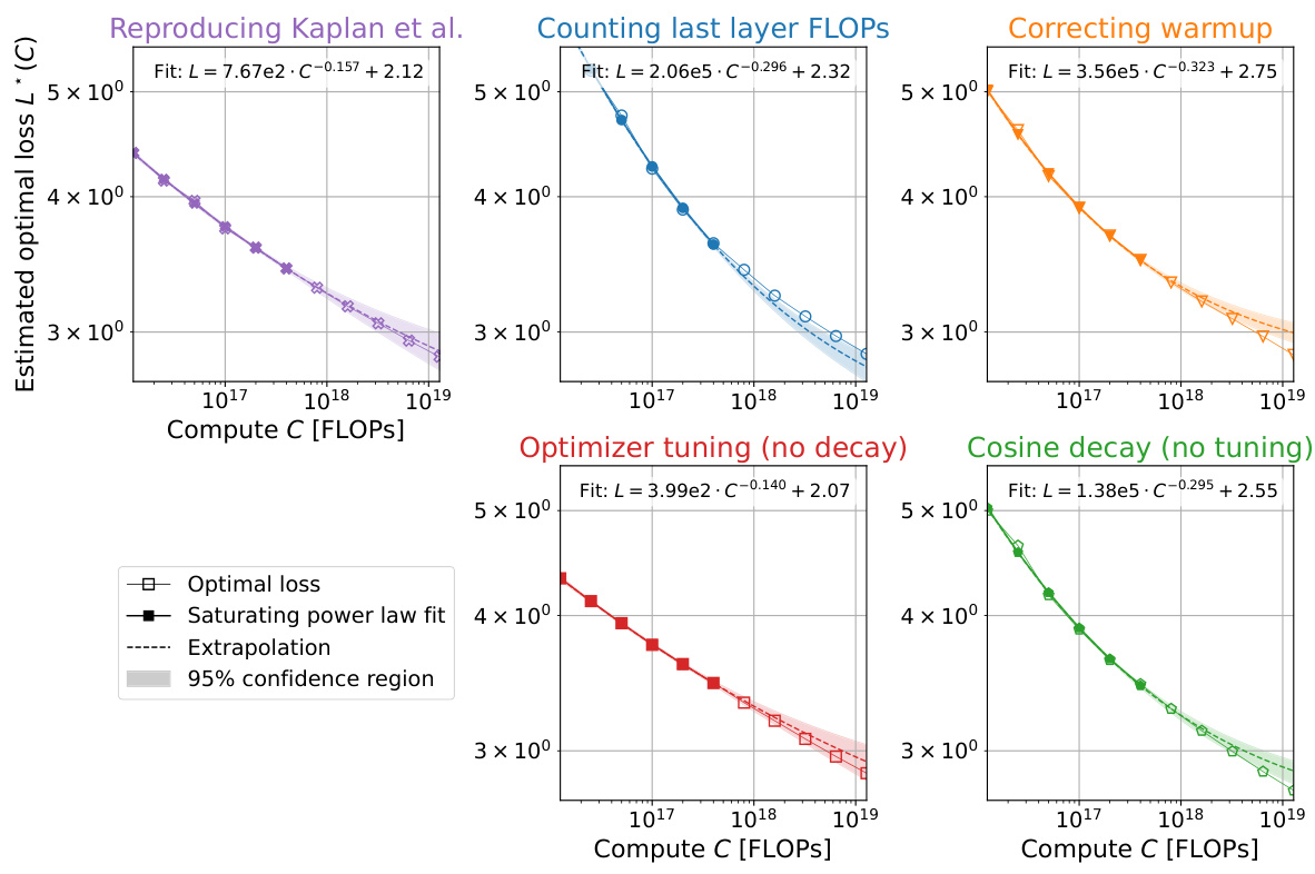
This figure shows the results of an experiment analyzing over 900 training runs to understand the discrepancies between the scaling laws proposed by Kaplan et al. and Hoffmann et al. Each panel displays the optimal model size (N*) plotted against the compute budget (C), along with power law fits to the data. By systematically adjusting different factors (last layer computational cost, warmup duration, and optimizer tuning), the authors demonstrate how the initial discrepancy between the two scaling laws can be resolved, ultimately showing strong agreement with Hoffmann et al.’s findings.
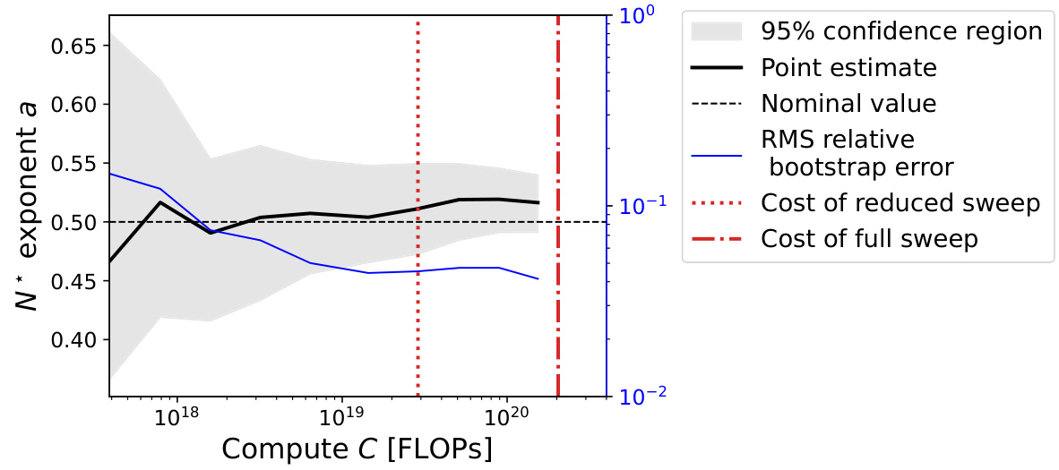
This figure displays a series of graphs that analyze the factors contributing to discrepancies between two influential scaling laws for language models (Kaplan et al. and Hoffmann et al.). It systematically reproduces Kaplan et al.’s findings and then isolates three key factors – last layer computational cost, warmup duration, and scale-dependent optimizer tuning – which explain the difference. By correcting these factors, the authors demonstrate excellent agreement with the Chinchilla scaling law. Each panel shows the optimal model size (N*) plotted against the compute budget (C), fitted with power laws, demonstrating how the corrections bring the two scaling laws into alignment.
More on tables
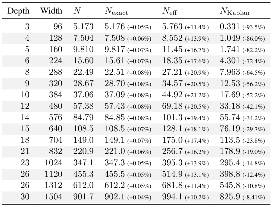
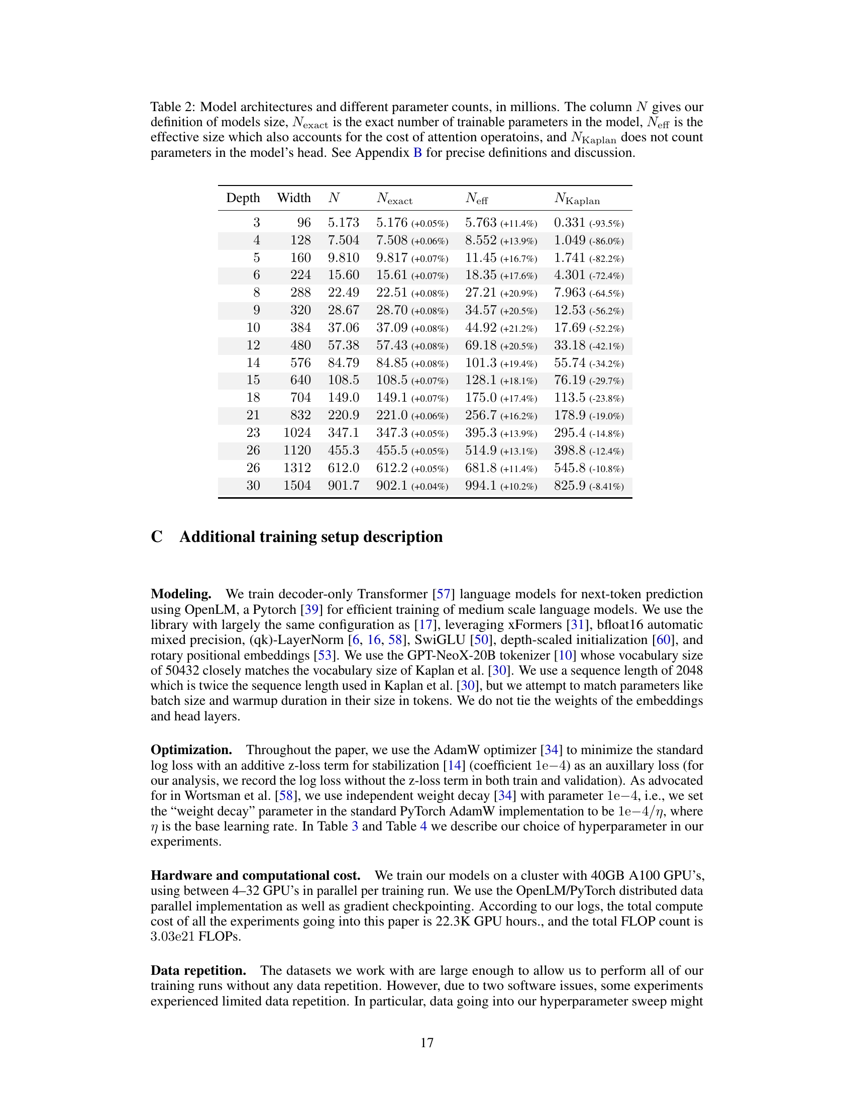
This table shows the model architectures used in the experiments, along with different ways to count the number of parameters in each model. N represents the number of parameters in all the linear layers (excluding embeddings, but including the head). Nexact counts all trainable parameters. Neff accounts for the computational cost of attention operations. Finally, NKaplan excludes parameters from the model’s head, as was done in the work by Kaplan et al. Appendix B provides a more detailed explanation of these variations and their implications.
This table shows the different ways to calculate the number of parameters of the language models used in the experiments. It compares four different metrics for parameter count: * N: The number of parameters in all linear layers (excluding embeddings but including the final linear layer). This is the primary definition used in the paper for the model size. * Nexact: The exact number of trainable parameters in the model. * Neff: An effective model size that also accounts for the computational cost of attention operations. * NKaplan: The parameter count that does not include the parameters in the model’s head (final linear layer). This method is used by Kaplan et al. [30] The table lists these counts for several model architectures that vary in depth and width. It provides the percentage differences between N and Nexact, N and Neff to demonstrate the magnitude of variations among the different parameter counting methods. More details on the different model size definitions and their implications are discussed in Appendix B.
This table presents the model architectures used in the experiments, along with various measures of model size. The column ‘N’ represents the primary model size definition used in the paper, based on the number of parameters in the linear layers (excluding embeddings but including the head). ‘Nexact’ gives the precise count of trainable parameters, ‘Neff’ includes the computational cost of attention operations, and ‘NKaplan’ excludes the parameters in the final (head) layer. Appendix B provides further details on these different definitions of model size and their implications for the results.
This table shows the different ways to count the number of parameters of the model and their effect on the final results. It compares four different metrics for measuring model size: N (the method used in the main paper), Nexact (the exact number of trainable parameters), Neff (the effective model size that accounts for both linear and attention layers), and NKaplan (the model size used by Kaplan et al. [30], that excludes embedding parameters and the model’s head). The table also shows the percentage difference between N and Nexact, N and Neff, and N and NKaplan. Appendix B provides a more detailed explanation of these metrics and their impact on the FLOP computation.

This table presents the different model architectures used in the experiments, along with various ways to calculate the number of parameters. N is the primary measure of model size used in the paper, excluding embedding layers, but including the final output layer (the head). Nexact includes all trainable parameters. Neff accounts for the computational cost of the attention mechanism. NKaplan excludes parameters in the head. The table shows how these values vary across different model sizes and depths and also indicates the relative percentage difference between N and these alternative metrics.
This table presents a comparison of different ways to measure the size of language models. It lists model architectures with varying depths and widths, and shows the number of parameters using three different methods: N (the authors’ definition of model size), Nexact (the exact number of trainable parameters), and NKaplan (which excludes parameters in the final layer). The table highlights the differences between these methods and explains their implications for computing the model’s computational cost. Appendix B provides further details on how these different methods of measuring model size are defined and why the authors chose their preferred definition (N).
Full paper#
