↗ OpenReview ↗ NeurIPS Proc. ↗ Hugging Face ↗ Chat
TL;DR#
Generating high-quality discrete data, like code or text, has been challenging for non-autoregressive models, which lag behind autoregressive counterparts. Existing methods struggle with high-dimensional discrete data, often relying on embedding techniques that compromise performance or are computationally expensive. This limitation hinders progress in various applications like code generation and language modeling.
This paper introduces Discrete Flow Matching (DFM), a novel framework addressing these challenges. DFM uses flexible probability paths and a generic sampling formula based on learned posteriors, achieving state-of-the-art performance on HumanEval and MBPP coding benchmarks as well as outperforming other models in text generation tasks. DFM also shows significant improvements by scaling up the model size, highlighting the scalability and potential for future enhancement of the approach.
Key Takeaways#
Why does it matter?#
This paper is crucial for researchers in AI and machine learning, particularly those working on generative models for discrete data. It bridges the performance gap between autoregressive and non-autoregressive models, offering a new approach with significant potential for improvement in tasks like code generation and language modeling. The framework presented opens new avenues of research into advanced discrete flow methods, potentially leading to more efficient and high-quality generative models.
Visual Insights#

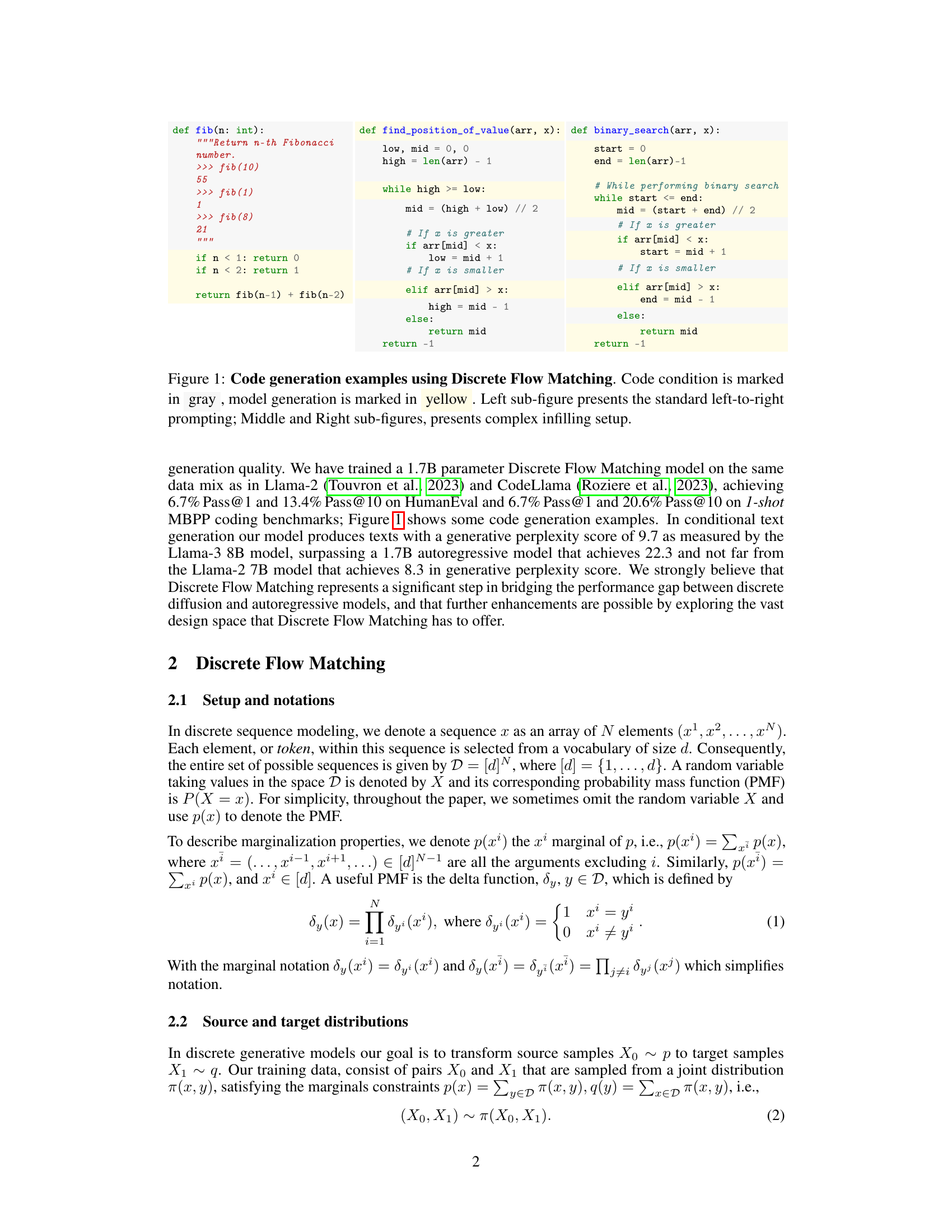
This figure shows examples of code generation using the Discrete Flow Matching model. The input code condition is shown in gray, and the model’s generated code is highlighted in yellow. The leftmost example demonstrates a standard left-to-right prompting approach, while the middle and right examples showcase more complex code infilling scenarios, where the model needs to fill in missing parts of the code within a more complex context.

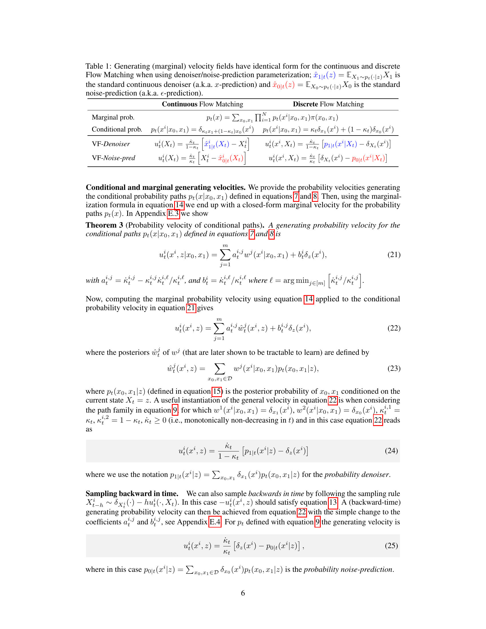
This table compares the formulas for generating velocity fields in continuous and discrete Flow Matching. It shows that the formulas are identical when using denoiser/noise-prediction parameterization. The table highlights the use of x-prediction (denoiser) and ε-prediction (noise-prediction) and how they relate to the marginal probability and conditional probability within both continuous and discrete frameworks.
In-depth insights#
Discrete Flow Match#
Discrete Flow Matching presents a novel approach to generative modeling for high-dimensional discrete data, a domain where traditional flow-based methods often underperform compared to autoregressive models. The core innovation lies in its ability to handle a general family of probability paths interpolating between source and target distributions, using a flexible formula for sampling. This flexibility is key, as it allows the model to leverage diverse learned posteriors such as probability denoisers or noise predictors. The authors demonstrate improved generative perplexity relative to previous discrete diffusion and flow models. Importantly, scaling up model parameters significantly enhances performance on coding tasks, highlighting the effectiveness of the approach for complex sequential data. The method cleverly unifies the theory and algorithm for probability path construction and corrector sampling, offering advancements over existing discrete flow approaches.
Prob Path & Vel#
The heading ‘Prob Path & Vel’ likely refers to the core methodology of a research paper focusing on probabilistic modeling, specifically on how to construct and utilize probability paths and their associated velocity fields to generate samples from a target distribution. The probability path represents a continuous transformation between a source distribution (often a simple distribution like uniform noise) and the target distribution (the data to be generated). The velocity field guides the sampling process along this path. Understanding the design and properties of probability paths (e.g., linear, quadratic, or more complex interpolations) is crucial for efficient sampling and achieving high-quality generated samples. Careful consideration of the velocity field ensures that the sampling process remains tractable and accurately reflects the target distribution. The effectiveness of this method likely depends on the appropriate choice of path and velocity function, and their interplay determines the speed and accuracy of the sampling, as well as the quality of the generated samples. The success of this approach hinges on the careful selection of probability paths and the ability to efficiently learn and utilize velocity fields.
Code Generation#
The research paper section on code generation showcases the model’s ability to produce functional code. The results demonstrate that the model outperforms existing non-autoregressive baselines on various benchmarks, significantly closing the gap between autoregressive and non-autoregressive approaches. Key to the model’s success is its use of Discrete Flow Matching, which improves generative perplexity, a key metric for code generation. The model exhibits impressive performance on complex coding tasks such as HumanEval and MBPP, indicating its capability to handle nuanced problems. Furthermore, the method is shown to generalize effectively to both standard left-to-right prompting as well as more complex infilling scenarios, highlighting its adaptability and practicality. While achieving state-of-the-art results on several benchmarks, the paper also acknowledges limitations, particularly in achieving the same level of sampling efficiency seen in continuous methods, which represents an exciting area for future research.
Future Work#
The ‘Future Work’ section of this research paper on Discrete Flow Matching presents exciting avenues for extending this novel approach. Scaling up model size and exploring more sophisticated architectural designs are key to bridging the performance gap between autoregressive and non-autoregressive models, particularly for more complex discrete data. Investigating different probability paths and corrector schedulers to optimize model training and improve sample quality is also crucial. A promising area is applying Discrete Flow Matching to diverse modalities beyond language and code, such as protein design, music generation, or time series data, leveraging the model’s non-autoregressive nature for improved efficiency. Finally, a deep dive into the theoretical underpinnings of the method, possibly with connections to continuous flow matching, will strengthen its foundation and reveal new avenues for advancement. Thorough investigation into the computational efficiency of the sampling process will be vital in making this technique more practical for real-world applications.
Limitations#
A thoughtful analysis of the limitations section of a research paper is crucial for a comprehensive understanding. The primary focus should be on identifying the shortcomings and constraints of the study’s methodology, scope, and results. It’s important to go beyond simply listing limitations and delve into their implications for the overall conclusions. For instance, if the study relies on a specific dataset, it’s essential to analyze how the characteristics of that dataset might limit the generalizability of the findings. Similarly, any assumptions made during the study, particularly in theoretical models, should be carefully evaluated, acknowledging potential biases or simplifications. Discussing the limitations of the used models or algorithms, including their computational complexity and potential vulnerabilities, can also uncover limitations. The aim is to provide a balanced assessment of the paper’s contribution, clearly acknowledging where the work falls short and how these limitations might impact future research. Examining these aspects with a critical eye can greatly improve the robustness and reliability of research.
More visual insights#
More on figures

This figure compares continuous and discrete flows. The left panel shows a continuous flow in RN (N=2), illustrating how probability changes smoothly in continuous space. The middle-left panel depicts a discrete flow in D = [d]N (d=4, N=2), where probability changes occur discretely between states. The rate of probability change, represented by divergence, is visualized in the middle-right and right panels for continuous and discrete scenarios, respectively. Divergence in the continuous case is a vector field illustrating the flow, while in the discrete case divergence is calculated between adjacent states using a difference operator.
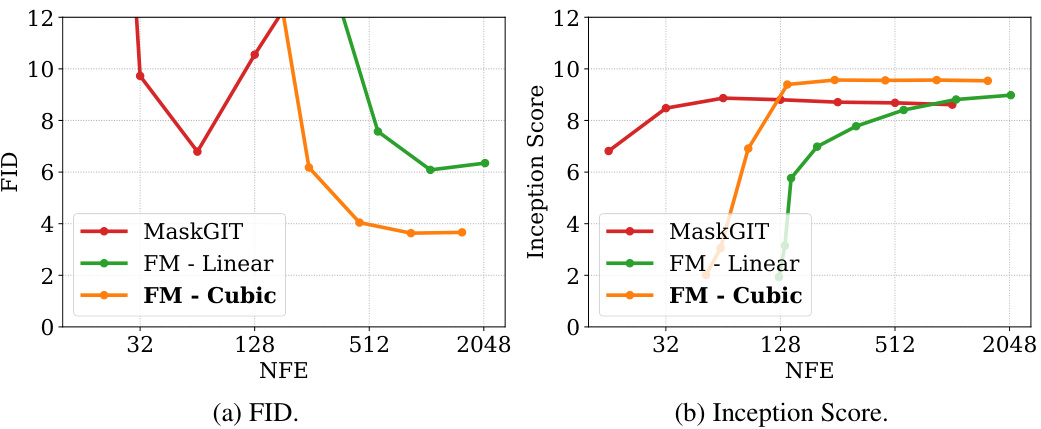
This figure compares the performance of different models on the task of image generation. The x-axis shows the number of function evaluations (NFE), which is a measure of computational cost. The y-axis shows two different metrics: the Fréchet Inception Distance (FID) and the Inception Score. Lower FID scores indicate better image quality. Higher Inception Scores indicate better image quality. The figure shows that Discrete Flow Matching (FM) with cubic scheduling outperforms both MaskGIT and FM with linear scheduling.

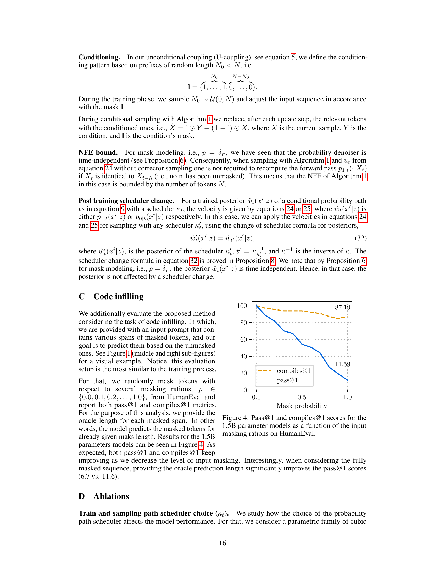
This figure shows the performance of the proposed model and autoregressive model on HumanEval and MBPP coding tasks. It presents the pass rate at different thresholds (Pass@1, Pass@10, Pass@25) for both text and code generation. The results demonstrate the ability of the Discrete Flow Matching model to generate high-quality code, approaching the performance of the autoregressive model. It also showcases a further improvement when the model is provided with the length of the solution (Oracle length).

This figure compares discrete and continuous flows. The left panel shows a continuous flow in RN, where N=2. The middle-left panel shows a discrete flow in D=[d]N, where d=4 and N=2. The rate of change in probability for a state (represented by a gray disk) is determined by the divergence operator. The middle-right and right panels illustrate this divergence operator in the continuous and discrete cases, respectively.

This figure illustrates the core concept of the paper: Discrete Flow Matching. It contrasts the continuous and discrete versions of flow matching. The left panel shows a continuous flow in RN (N=2 here, so a 2D space), depicting how probability flows in this continuous space. The middle-left panel visualizes discrete flow in D = [d]N (a discrete space, with d=4 and N=2). This panel highlights the differences in how probability changes. Both versions use divergence operators (right panels) to track the rate of probability change in their respective spaces. The key is showing how the theoretical framework adapts continuous flow concepts to discrete spaces.
This figure compares discrete and continuous flows. The left side shows a continuous flow in RN, illustrating the concept of divergence using a gray disk representing a state’s probability. The middle-left shows a discrete flow in D = [d]N with d=4 and N=2, highlighting the discrete nature of state transitions. The middle-right and right panels illustrate how probability changes are represented differently in continuous (divergence) and discrete settings. This visualization helps understand the core difference between continuous and discrete flow matching approaches.

This figure shows the Fréchet Inception Distance (FID) scores on the CIFAR10 dataset for different training and evaluation schedulers. The four schedulers compared are Linear, Quadratic, Cubic, and Cosine. The heatmap visualizes the FID scores, where each cell represents the FID achieved when a model trained with one scheduler is evaluated using another. The absence of corrector sampling and a temperature of 1 are noted.
More on tables

This table compares the formulas for generating velocity fields in both continuous and discrete Flow Matching. It highlights that the formulas are remarkably similar when using denoiser/noise-prediction parameterization. The table shows the marginal probability, conditional probability, velocity field formulas using denoiser and noise prediction for both continuous and discrete settings.

This table compares the generative perplexity of various language models on unconditional text generation. It shows the performance of the proposed Discrete Flow Matching (FM) models against several autoregressive and other non-autoregressive baselines. The metrics include perplexity scores calculated using Llama-2, Llama-3, and GPT-2, as well as entropy, which reflects token diversity. The number of function evaluations (NFE) is also indicated for each model, representing the computational cost. Note that results for double precision sampling are presented in a separate table (Table 5).

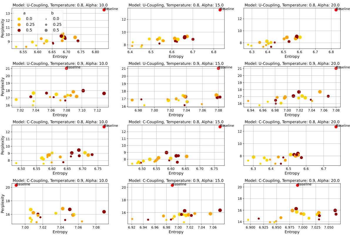
This table compares the generative perplexity of different language models on conditional text generation tasks. It shows the performance of Llama-2 and Llama-3 (used as references), an autoregressive model, and the Discrete Flow Matching (FM) model with both unconditional (U-coupling) and conditional (C-coupling) strategies. The results are presented for different model sizes and numbers of function evaluations (NFEs). Lower perplexity scores indicate better performance.

This table presents the results of code generation experiments on HumanEval and MBPP benchmarks. It compares the performance of an autoregressive model against the Discrete Flow Matching (FM) model proposed in the paper. The evaluation metrics are Pass@k (percentage of correctly generated codes within k attempts). The table is broken down by data type (text and code), and the FM results are further separated into results with and without oracle length (i.e., with or without knowledge of the correct code length). Higher Pass@k values indicate better performance.

This table compares the generative perplexity of various language models on unconditional text generation tasks. The models include both autoregressive and non-autoregressive approaches. The perplexity is measured using different evaluation models (LLAMA-2, LLAMA-3, GPT2), and the number of function evaluations (NFE) is also reported. Note that temperature and corrector steps are not used during sampling for these results. A more detailed comparison including double precision sampling is available in Table 5.
Full paper#
