↗ OpenReview ↗ NeurIPS Proc. ↗ Hugging Face ↗ Chat
TL;DR#
Large language model (LLM) training is computationally expensive, and current research relies heavily on the cosine learning rate schedule, which is suboptimal because it requires training models for different lengths. This creates needless complexity in scaling experiments and makes scaling research less accessible and more expensive. This paper addresses these issues. The paper proposes a simpler alternative: a constant learning rate with a cooldown period at the end of training. This approach removes the need to train multiple models for different durations and makes scaling experiments much cheaper. It also shows that stochastic weight averaging (SWA) improves model performance without added costs.
The authors conducted extensive experiments using this novel method and compared the results with cosine. They found that the constant learning rate with cooldown produced similar performance to cosine but at a drastically reduced computational cost. The incorporation of SWA further improved performance. Their findings demonstrate that large-scale scaling experiments can be performed much more cheaply with fewer training runs. The authors release their code to promote wider adoption and replication, further driving research and development in the field of LLM training. This has significant implications for researchers with limited resources and for advancing the field as a whole by making large-scale research more accessible and affordable.
Key Takeaways#
Why does it matter?#
This paper significantly reduces the computational cost of large language model scaling experiments by showing that a simple alternative to the commonly used cosine learning rate schedule, namely a constant learning rate with cooldown, works equally well and allows for more flexible and efficient experiments. This is crucial for advancing the field, as it opens up new avenues for researching scaling laws with reduced compute costs and makes the field more accessible to researchers with limited resources.
Visual Insights#
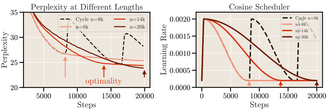
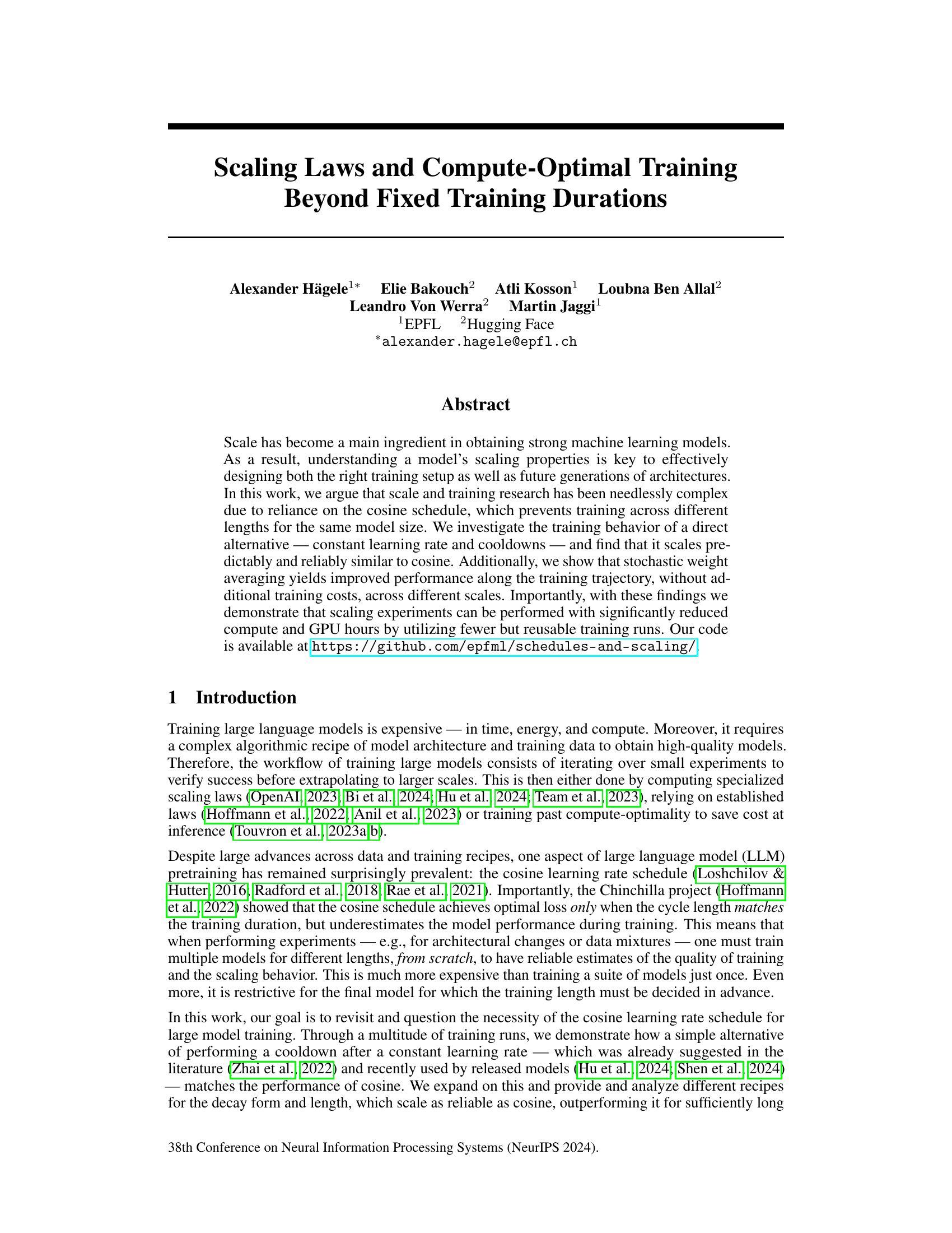
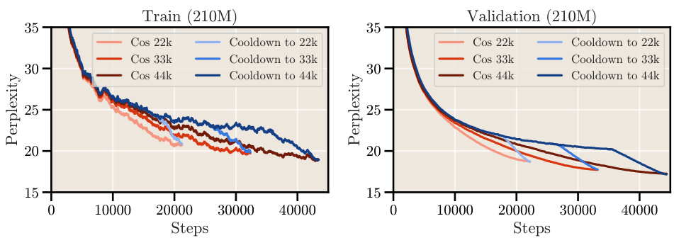
This figure shows that to achieve optimal performance with a cosine learning rate schedule, the total training duration must match the cycle length. The left panel shows that for different training lengths, the optimal perplexity is only achieved when the cycle length of the cosine schedule matches the training duration. The right panel shows the corresponding learning rate schedules used for each of these training durations. This limitation of the cosine schedule motivates the exploration of alternative scheduling techniques presented in Section 3 of the paper.
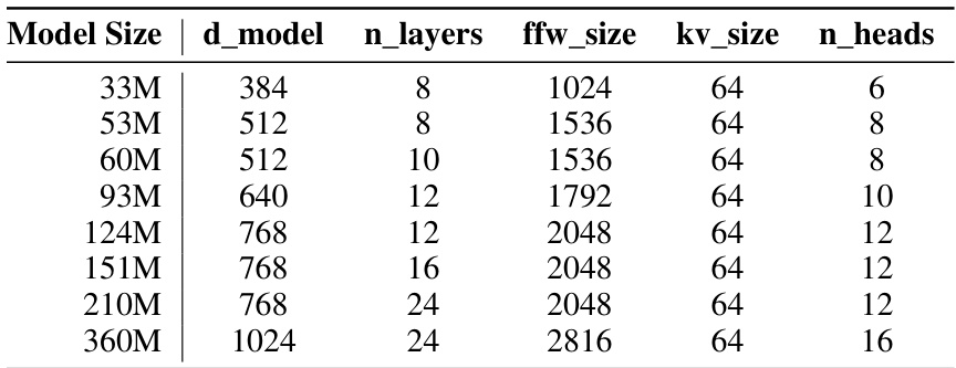
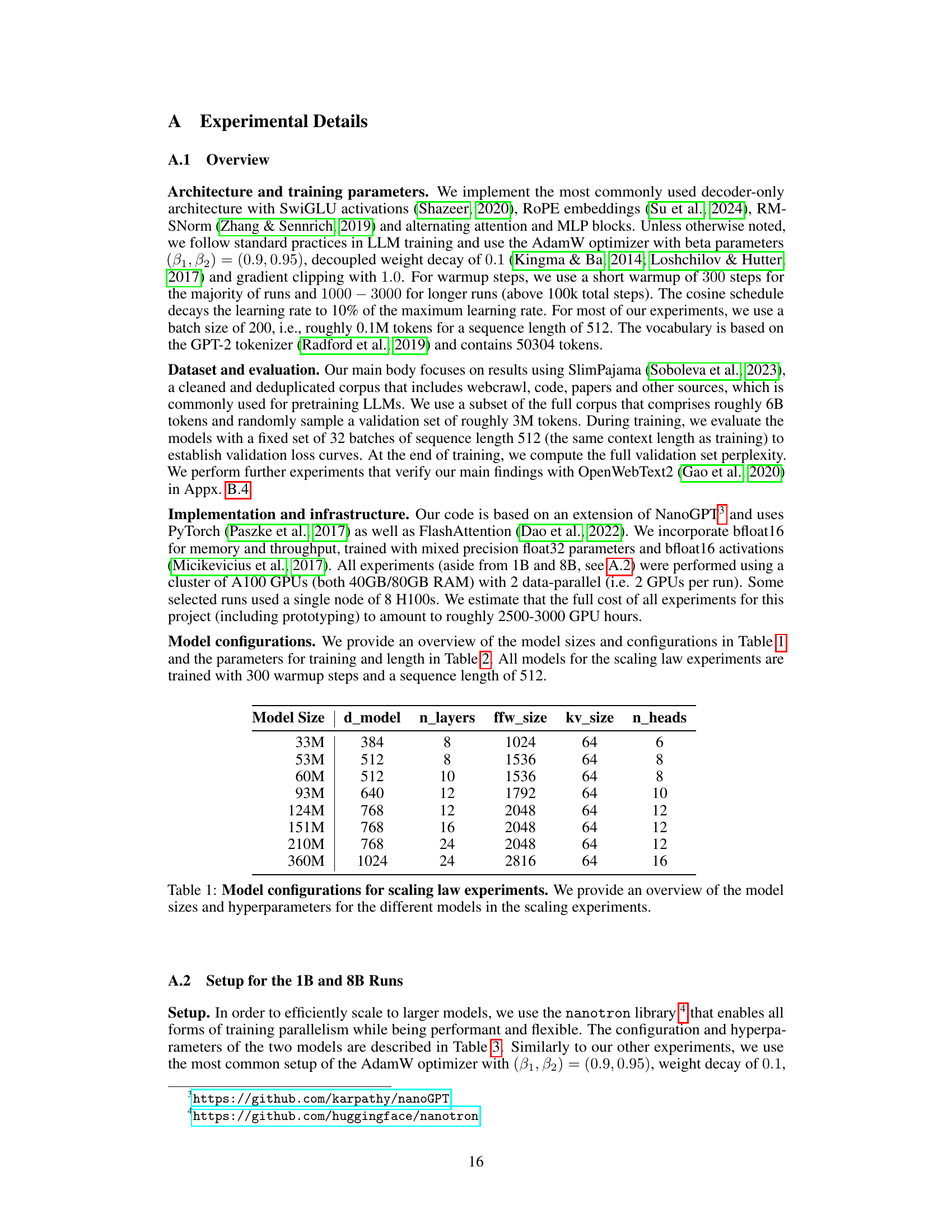
This table lists the configurations of the different transformer models used in the scaling experiments. For each model size (33M, 53M, …, 360M), it shows the values of several hyperparameters: the embedding dimension (d_model), the number of layers (n_layers), the feed-forward network size (ffw_size), the key/value vector size (kv_size), and the number of attention heads (n_heads). These hyperparameters directly impact the model’s capacity and computational cost.
In-depth insights#
Cosine Schedule Revisited#
The section ‘Cosine Schedule Revisited’ would delve into the widely used cosine learning rate schedule in large language model (LLM) training. It would likely begin by highlighting the schedule’s popularity and prevalent use, acknowledging its role in achieving state-of-the-art results in prominent LLMs. However, the analysis would then critically examine the limitations of this approach, possibly focusing on its dependence on pre-defining the training length to match the cosine cycle for optimal performance. This constraint is problematic for scaling experiments and flexible training. The section might present alternative scheduling strategies that overcome this limitation, perhaps by exploring methods that allow training for various durations without compromising performance. This could involve comparing constant learning rates with cooldown phases against cosine schedules, evaluating both their performance and computational efficiency. Ultimately, the section should offer a nuanced perspective, highlighting the strengths of cosine schedules while emphasizing the advantages of more flexible alternatives, thereby contributing to improved LLM training practices.
Cooldown Training#
The concept of “cooldown training” in the context of large language model (LLM) training offers a compelling alternative to traditional cosine annealing schedules. Instead of gradually decreasing the learning rate throughout the entire training process, cooldown training maintains a constant learning rate for a significant portion, followed by a sharp decrease in a relatively short final phase. This approach simplifies the training process, eliminating the need to pre-define the total training duration, as the cooldown can be initiated at any time. Furthermore, this method appears to scale predictably and reliably across different model sizes. The authors’ experiments indicate that using a constant learning rate with a strategically-placed cooldown phase results in similar or better model performance as cosine scheduling, while enabling substantial computational savings. The study highlights the advantages of this approach in the context of scaling law experiments, allowing for more efficient and cost-effective model evaluations.
SWA: An Alternative#
The concept of using Stochastic Weight Averaging (SWA) as an alternative training approach in large language models (LLMs) presents a compelling avenue for improvement. SWA offers a way to potentially enhance model generalization without the need for explicit learning rate decay schedules like cosine annealing. The authors explore SWA as a replacement for the cooldown phase, showing that it boosts performance, particularly when combined with a constant learning rate. While SWA doesn’t fully close the performance gap compared to models trained with explicit cooldown phases, it provides a significant benefit by improving generalization with minimal computational overhead. This makes it an attractive alternative for researchers seeking more efficient and reliable LLM training, especially when considering the practical challenges of tuning complex learning rate schedules. The absence of a need for meticulously tuned LR decay makes SWA particularly attractive for large-scale experiments and scaling law research. By utilizing SWA, researchers could significantly reduce the computational resources needed for these experiments, as training from scratch for multiple schedules is not required. Further research is needed to fully understand its capabilities and limitations within different LLM architectures and training regimes.
Scaling Law Efficiency#
Scaling laws in large language models (LLMs) reveal crucial relationships between model size, dataset size, and performance. However, empirically deriving these laws is computationally expensive, requiring numerous training runs across different scales. This paper significantly improves the efficiency of scaling law experiments by proposing a novel training schedule. Instead of using the conventional cosine learning rate schedule, which necessitates separate runs for each desired training duration, the authors introduce a constant learning rate with cooldown approach. This dramatically reduces the need for repeated training runs because the cooldown phase can be initiated retrospectively at any point, providing reliable performance estimates without retraining from scratch. The method’s effectiveness is demonstrated through extensive experiments, resulting in considerable compute and GPU hour savings. This improved efficiency not only accelerates scaling law research but also makes it more accessible by significantly lowering the computational barrier to entry. Stochastic Weight Averaging (SWA) further enhances the approach’s practicality, boosting generalization and yielding better results. The proposed methods offer a significant advancement in LLM research, empowering more frequent and in-depth exploration of scaling properties.
Future Research#
Future research directions stemming from this work could explore more sophisticated cooldown schedules, potentially incorporating adaptive methods that dynamically adjust the decay rate based on model performance. Investigating the interaction between different cooldown functions and various optimizers beyond AdamW would also be valuable, potentially revealing new combinations that further enhance training efficiency. A thorough analysis of the generalizability of findings across diverse model architectures and datasets is crucial, as is extending the scaling law experiments to even larger models. Finally, research focusing on the interplay between cooldown strategies and techniques like stochastic weight averaging (SWA) promises to unlock further improvements in model performance and reduce computational costs.
More visual insights#
More on figures
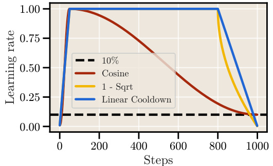
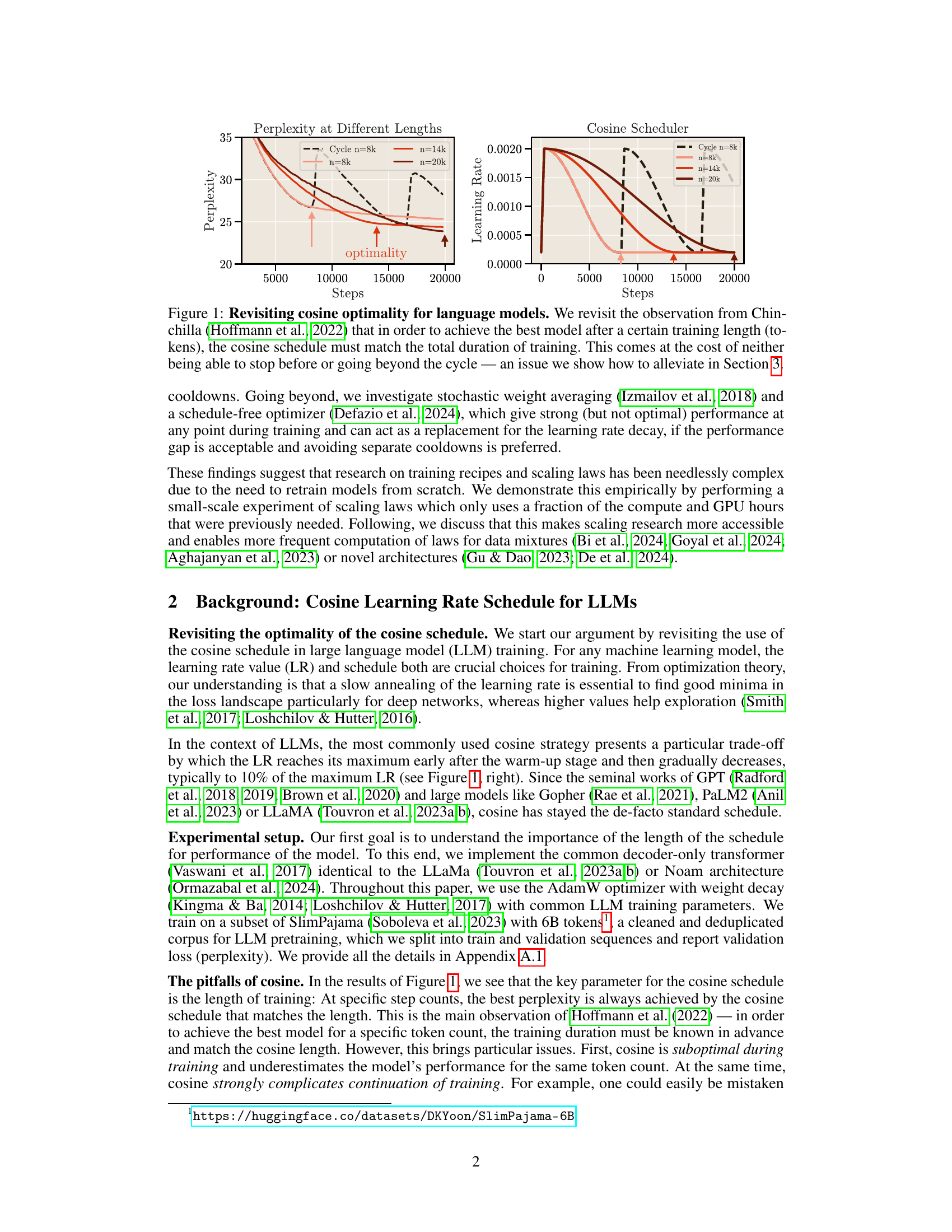
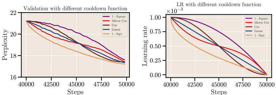
The figure compares different learning rate schedules used in training large language models. It shows the cosine schedule, which gradually reduces the learning rate over a long period, and two alternative schedules that use a constant learning rate followed by a sharp cooldown (linear and square root). The plot illustrates the different shapes of these schedules and how they vary over a certain number of training steps.
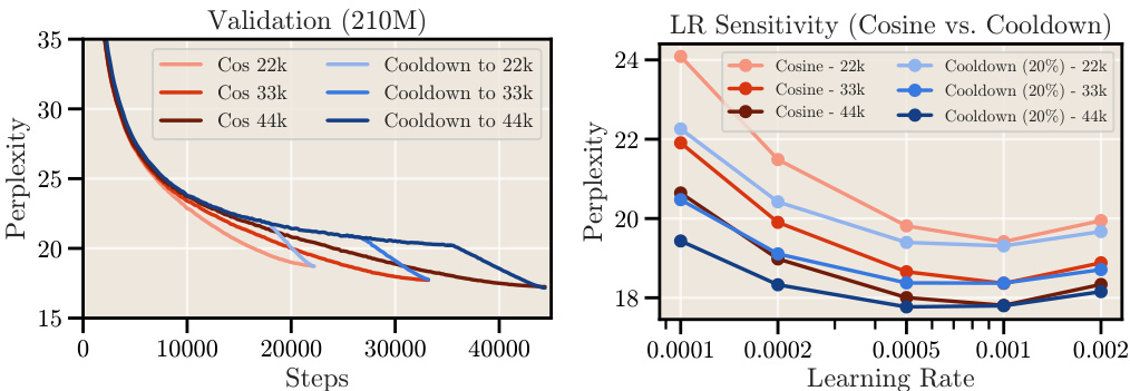
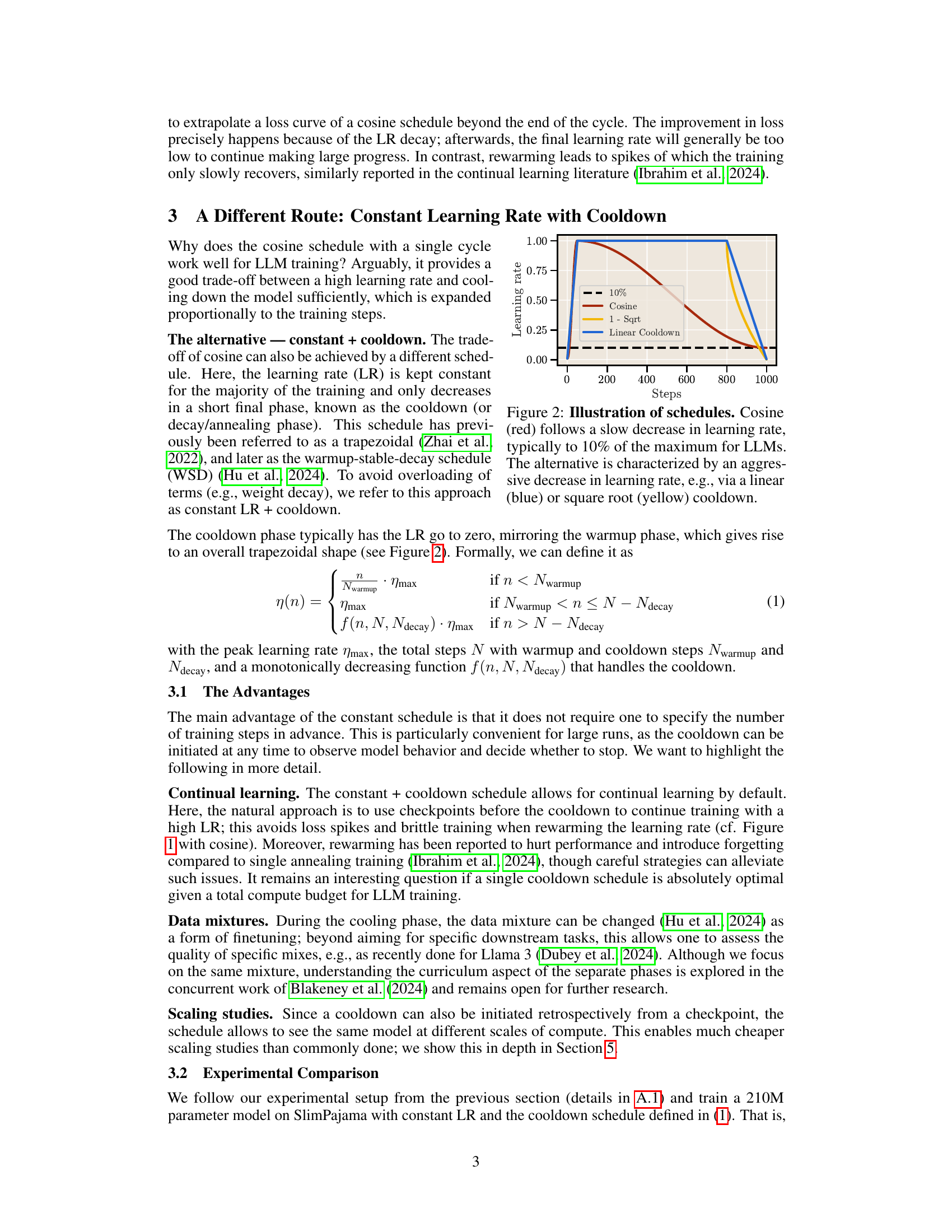
This figure compares the performance of the cosine learning rate schedule with a constant learning rate schedule that incorporates a cooldown phase. The left panel shows the loss curves for both schedules, demonstrating that the cooldown schedule achieves a similar sharp decrease in loss as the cosine schedule. The right panel shows the learning rate sensitivity for both schedules, indicating that the cooldown schedule is less sensitive to variations in the learning rate. The optimal learning rate for the cooldown schedule is slightly lower than the optimal learning rate for the cosine schedule.
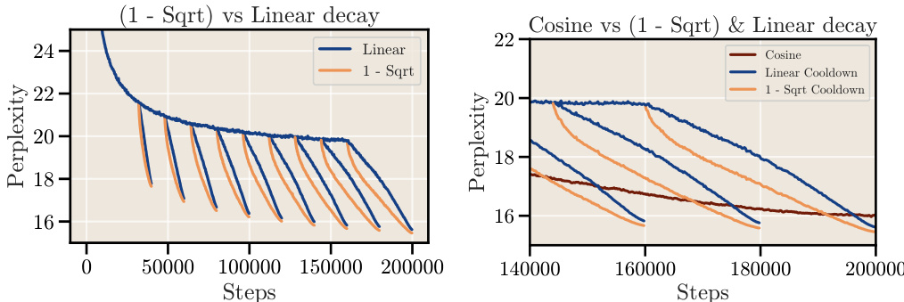
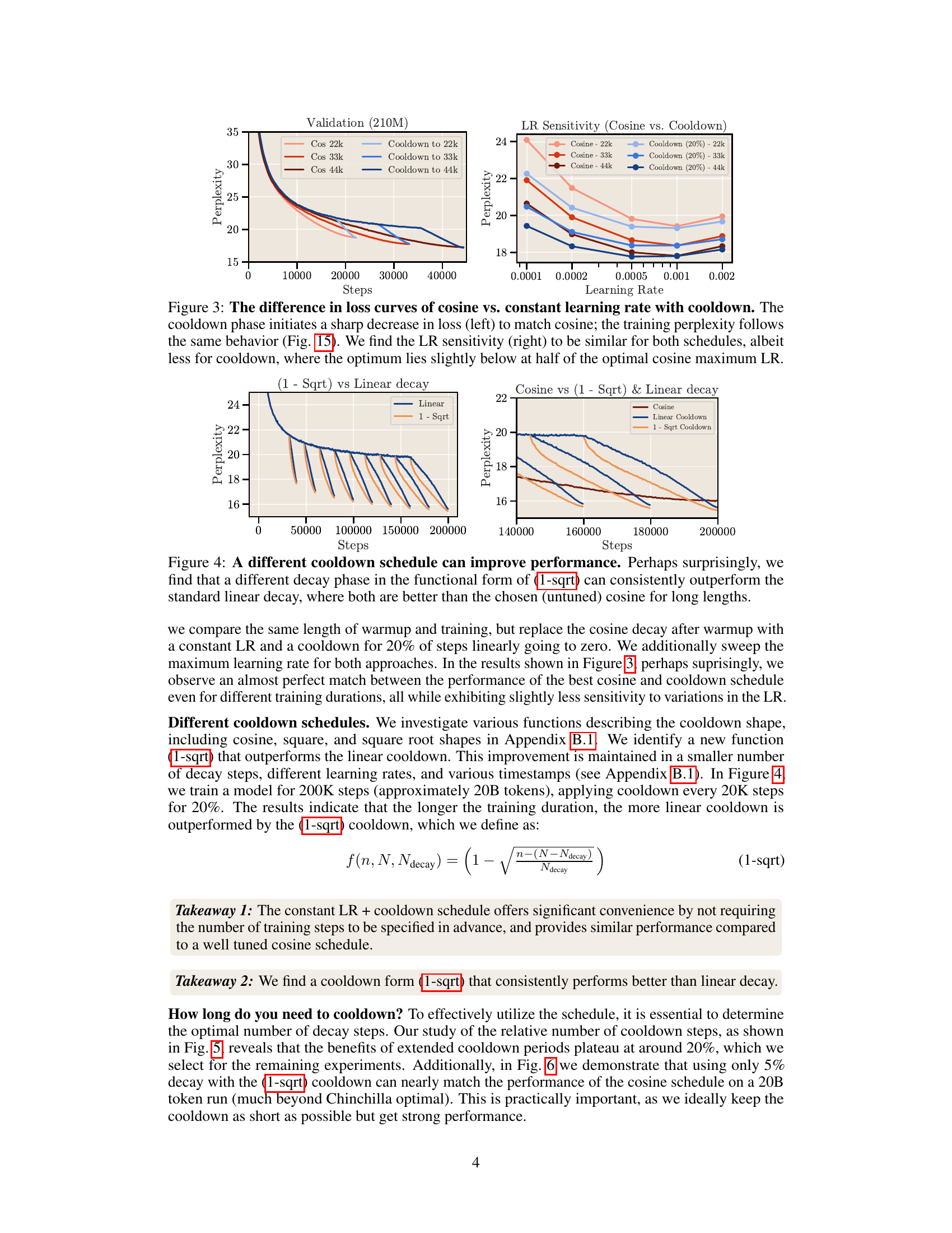
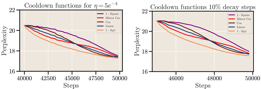
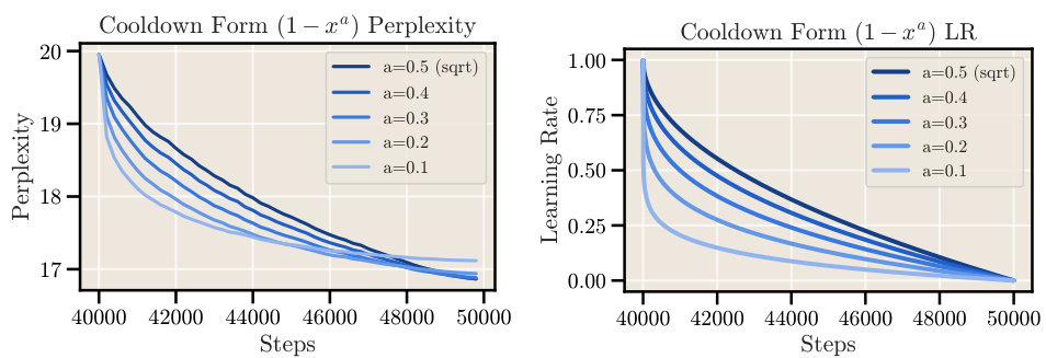
This figure compares the performance of different cooldown schedules (linear and 1 - sqrt) against the cosine schedule for long training durations. The results show that a square root decay function (1-sqrt) consistently outperforms the linear decay function, and both outperform the cosine schedule, especially for longer training runs.
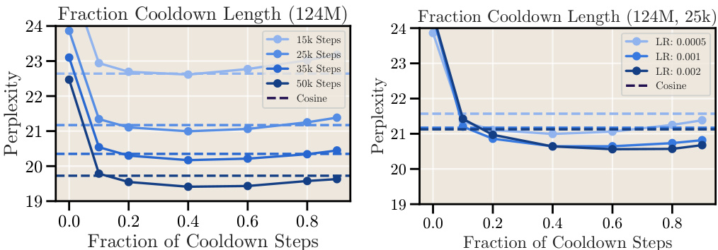
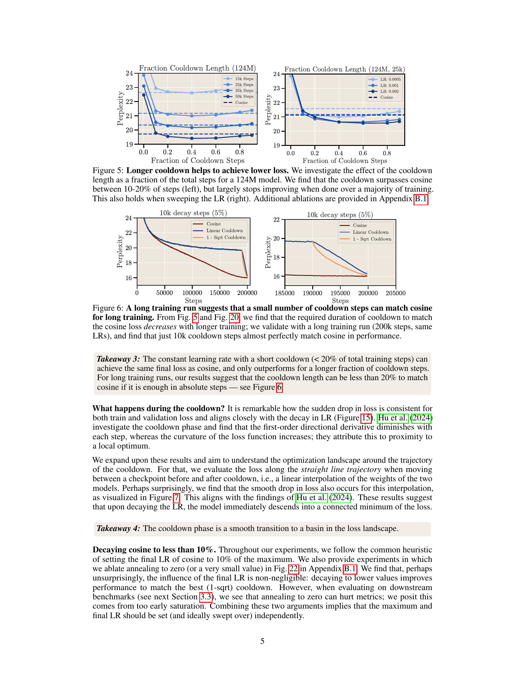
This figure shows the relationship between the cooldown length (as a fraction of total training steps) and the final loss (perplexity) achieved for a 124M parameter model. The left panel shows that increasing the cooldown length to 10-20% of the total training steps significantly improves the model’s performance, surpassing the cosine schedule’s performance. However, increasing the cooldown beyond this point does not result in further improvement. The right panel demonstrates the robustness of this finding by showing similar results across different learning rates.

This figure shows the results of a long training run (200k steps) comparing the performance of a constant learning rate with a short cooldown (10k steps, which is 5% of the total steps) against the cosine learning rate schedule. The results show that a short cooldown is sufficient to match the performance of the cosine schedule for long training runs, confirming the findings from previous figures (5 and 20) that the needed cooldown duration shrinks with longer training durations.
This figure compares the loss curves and learning rate sensitivity of two learning rate schedules: cosine and constant learning rate with cooldown. The left panel shows that the cooldown schedule achieves a sharp decrease in loss similar to the cosine schedule, while maintaining similar perplexity. The right panel demonstrates that the optimal learning rate for both schedules is comparable, with the cooldown schedule exhibiting slightly lower sensitivity to changes in the learning rate.
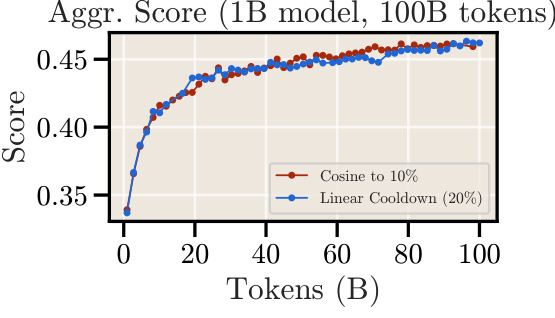
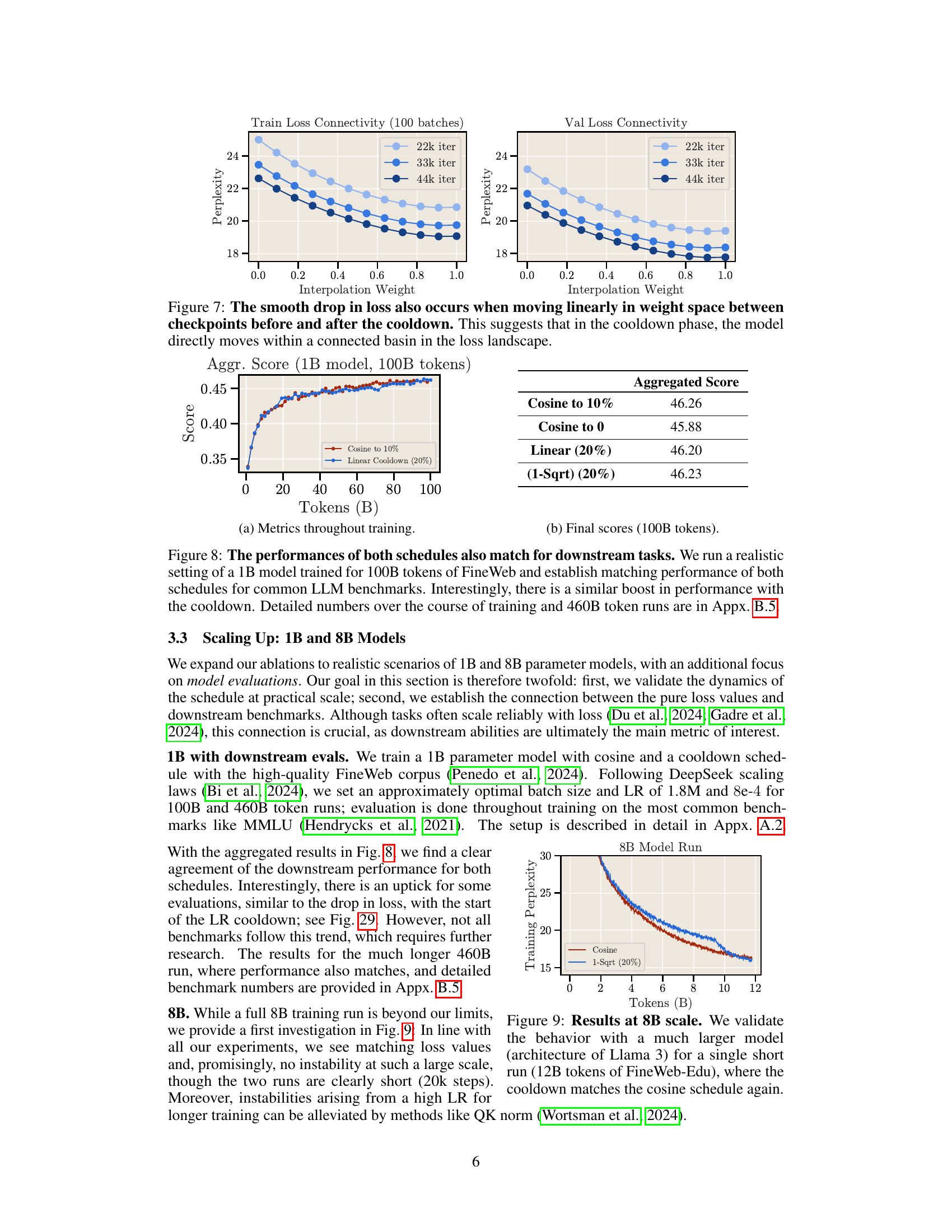
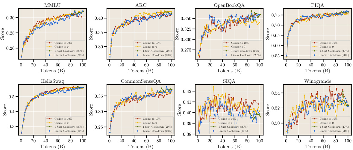
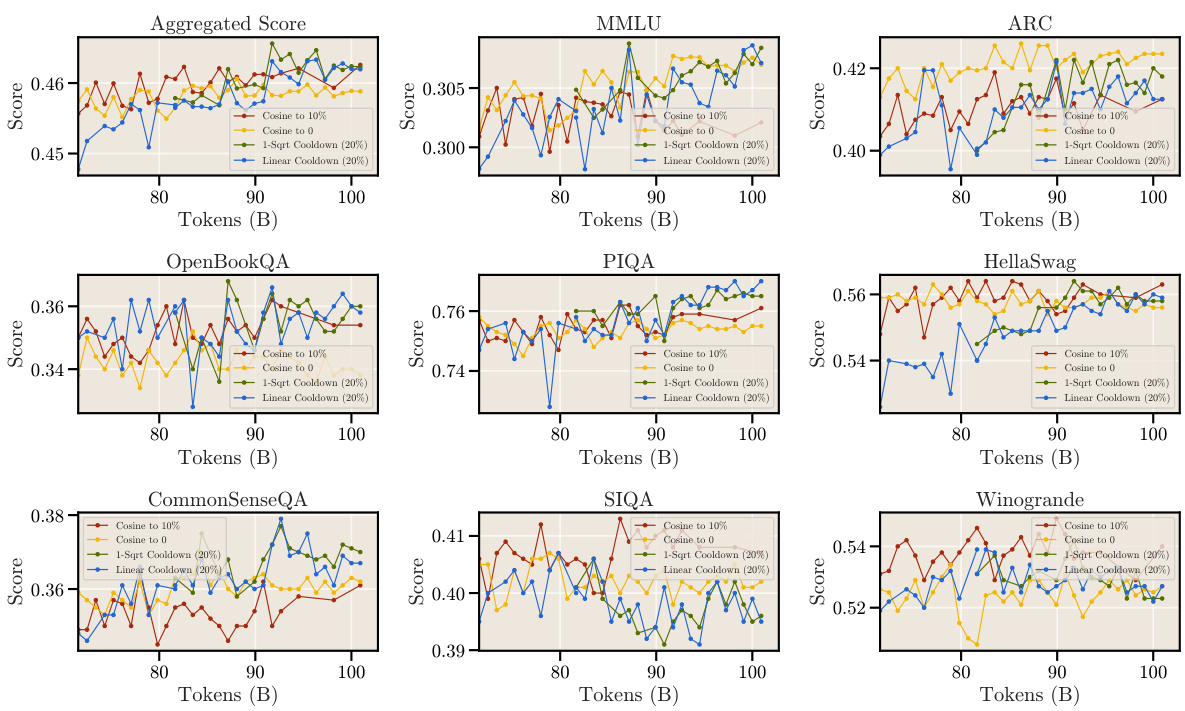
This figure compares the performance of cosine and linear cooldown schedules on a 1B parameter model trained with 100B tokens from the FineWeb dataset. The left subplot shows the aggregated score across various downstream tasks throughout the training process. The right subplot shows the final aggregated scores for both schedules after 100B tokens. The results indicate that both schedules achieve comparable performance on downstream tasks, with a potential performance boost observed at the beginning of the cooldown phase.
The figure compares two learning rate schedules: cosine and constant learning rate with cooldown. The left panel shows the loss curves, demonstrating that the cooldown schedule achieves a similar sharp decrease in loss as the cosine schedule, resulting in comparable training perplexity. The right panel illustrates that both schedules have similar sensitivities to changes in learning rate, however, the cooldown schedule’s optimal learning rate is slightly lower than that of the cosine schedule.
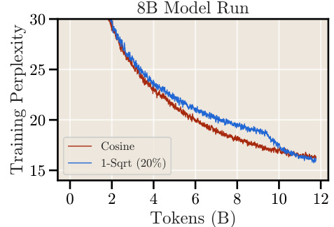
This figure shows the training perplexity curves for an 8B parameter model trained on 12B tokens of the FineWeb-Edu dataset. Two learning rate schedules are compared: a cosine schedule and a 1-sqrt cooldown schedule (where the cooldown constitutes 20% of the total training steps). The results demonstrate that the 1-sqrt cooldown schedule achieves a comparable final training perplexity to the cosine schedule, even for this much larger model size. This finding supports the authors’ claim that the 1-sqrt cooldown is a reliable alternative to the cosine schedule for training large language models, regardless of model size.
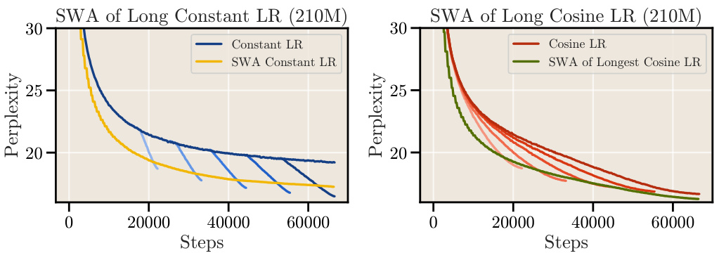
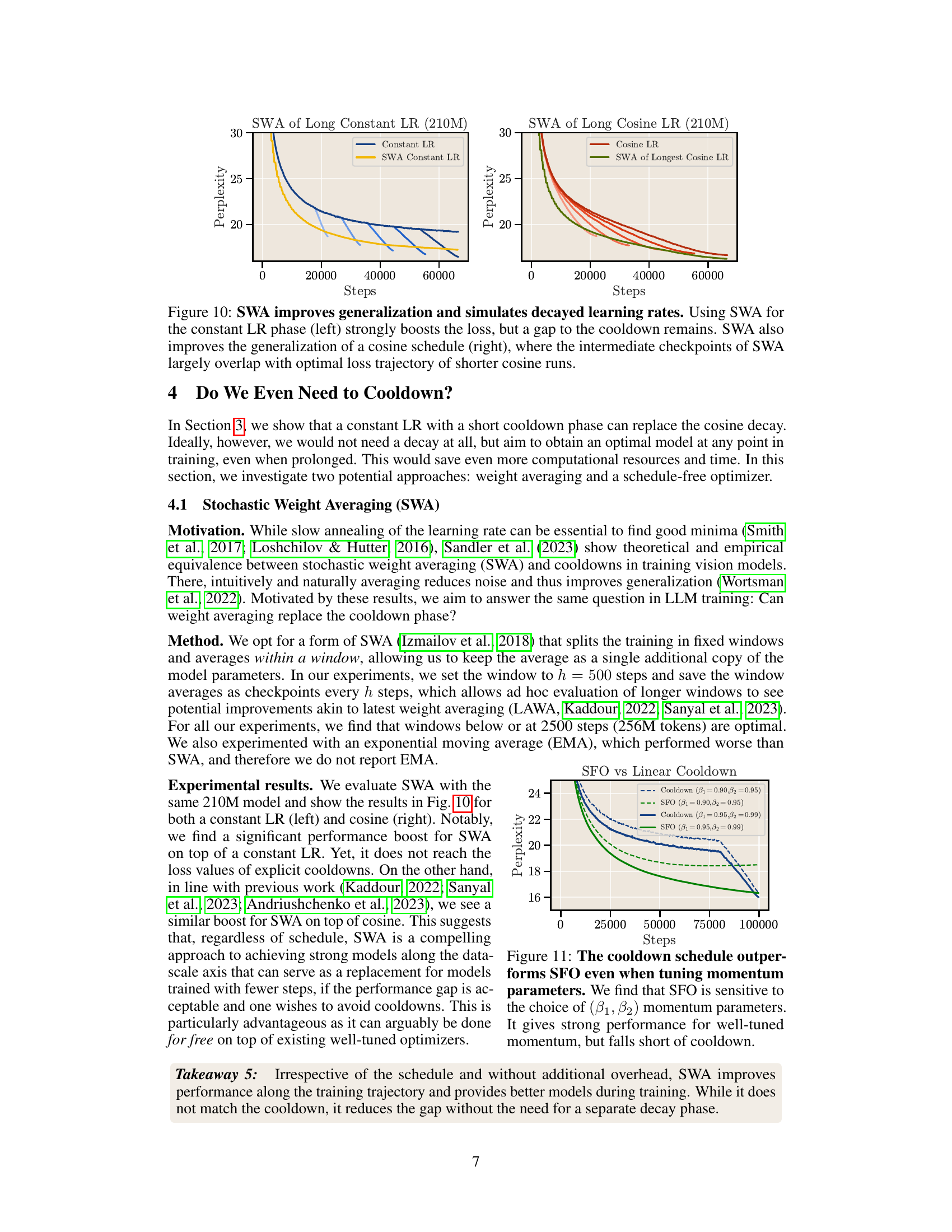
This figure shows the effect of Stochastic Weight Averaging (SWA) on two different learning rate schedules: a constant learning rate with cooldown and a cosine learning rate schedule. The left panel demonstrates that applying SWA to a constant learning rate schedule significantly improves the model’s performance, though it doesn’t fully close the gap to the performance achieved with the explicit cooldown. The right panel shows that SWA also improves the performance of a cosine learning rate schedule, with the SWA checkpoints closely tracking the optimal loss trajectory of shorter cosine training runs. This suggests that SWA acts as a form of implicit learning rate decay.
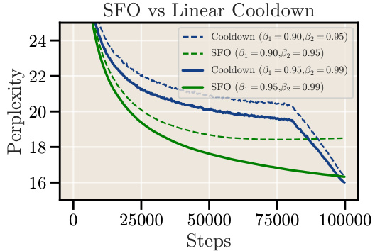
This figure compares the performance of a schedule-free optimizer (SFO) with a linear cooldown schedule for a 210M parameter language model. Two different momentum parameter settings ((β₁, β₂) = (0.90, 0.95) and (β₁, β₂) = (0.95, 0.99)) are used for both the SFO and linear cooldown to assess the impact of these parameters on performance. The graph plots perplexity against training steps, showing that, regardless of the momentum setting, the linear cooldown always yields lower perplexity (better performance) than the SFO.

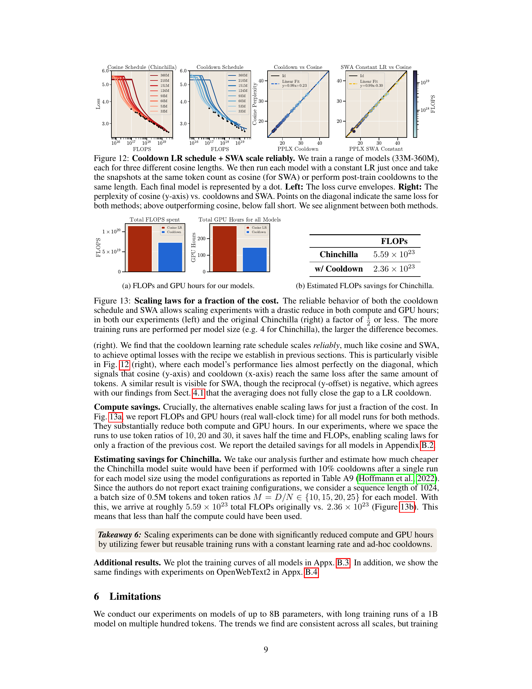
This figure demonstrates the scalability and reliability of the cooldown learning rate schedule and stochastic weight averaging (SWA) in comparison to the cosine schedule. It shows that models trained using the constant learning rate with cooldown or SWA achieve similar performance to those trained with the cosine schedule, with the cooldown method often outperforming cosine. The left panel displays loss envelopes for various model sizes, showing similar trends across methods. The right panel compares cosine perplexity against cooldown and SWA perplexity, highlighting that models trained with either alternative reach similar performance to cosine-trained models for the same FLOPs.

This figure compares the computational cost (FLOPs and GPU hours) of scaling experiments using the cosine schedule (Chinchilla’s approach) versus the proposed cooldown schedule and stochastic weight averaging (SWA). The left panel shows the results from the authors’ experiments, demonstrating a significant reduction in both FLOPs and GPU hours when using the cooldown/SWA methods. The right panel illustrates the potential savings for the original Chinchilla experiments, further highlighting the efficiency gains.
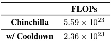
This figure demonstrates the significant reduction in computational cost achieved by using the proposed cooldown schedule and stochastic weight averaging (SWA) in scaling law experiments. The left panel shows the computational savings (FLOPS and GPU hours) for the experiments conducted in the paper, while the right panel illustrates the savings compared to the original Chinchilla experiments. It highlights that the proposed methods substantially reduce the computational requirements for scaling experiments by requiring fewer, reusable training runs.
This figure compares the loss curves and learning rate sensitivity of two learning rate schedules: cosine and constant learning rate with cooldown. The left panel shows that the cooldown phase in the constant learning rate schedule causes a sharp decrease in loss, similar to the behavior observed with the cosine schedule. The right panel shows that the optimal learning rate for both schedules is comparable, but the constant learning rate schedule with cooldown exhibits slightly less sensitivity to variations in learning rate and its optimal value is about half the maximum cosine learning rate.
This figure compares the loss curves and learning rate sensitivity of two learning rate schedules: cosine annealing and constant learning rate with cooldown. The left panel shows that the cooldown schedule produces a sharp decrease in loss, comparable to the cosine schedule. The right panel demonstrates that the optimal learning rate for both schedules is similar, but the constant learning rate with cooldown shows slightly less sensitivity, with the optimum learning rate being around half of the cosine schedule’s optimal maximum learning rate.
This figure compares the loss curves and learning rate sensitivity of two different learning rate schedules: cosine and constant learning rate with cooldown. The left panel shows that both schedules achieve a similar sharp decrease in loss during the cooldown phase. The right panel demonstrates that both schedules exhibit similar sensitivity to the learning rate, although the optimal learning rate for the cooldown schedule is slightly lower than that of the cosine schedule.
This figure shows that the cosine learning rate schedule achieves optimal loss only when its cycle length matches the training duration. It highlights the problem that stopping training before or extending it beyond the cycle leads to suboptimal results. The authors illustrate how a constant learning rate with cooldown addresses this limitation.
The figure shows two plots. The left plot shows the perplexity versus steps for different cycle lengths using the cosine scheduler. It demonstrates that the cosine scheduler only reaches optimality when the cycle length matches the total training duration. The right plot shows the learning rate versus steps for different cycle lengths using the cosine scheduler. It highlights that the learning rate decreases gradually with training steps, reaching its minimum value at the end of the cycle. This behavior demonstrates the limitation of cosine schedulers in terms of flexibility and ability to achieve optimality across different training lengths.
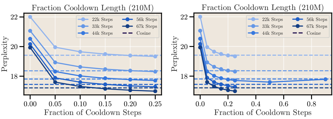
This figure shows the relationship between the length of the cooldown phase and the final perplexity achieved during training for a 210M parameter language model. The experiment was repeated from Figure 5 but with a 210M parameter model. The x-axis represents the fraction of training steps dedicated to the cooldown phase, and the y-axis represents the final perplexity. It shows that there’s an optimal cooldown length that minimizes the perplexity, and that extending the cooldown beyond this point does not further improve the results. A zoomed-in view is presented on the left for better visualization of the optimal range.
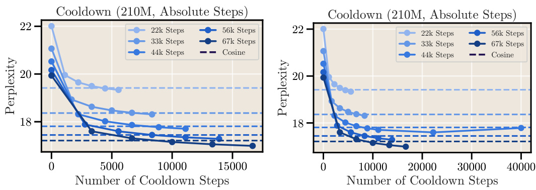
This figure shows the relationship between the length of the cooldown period and the final perplexity achieved by a 210M parameter language model. The left panel shows a zoomed-in view of the relationship, while the right panel provides a broader overview. The results suggest a parabolic relationship, where increasing the cooldown length initially improves performance but then leads to diminishing returns.

This figure compares the loss curves and learning rate sensitivity of two learning rate schedules: cosine annealing and constant learning rate with cooldown. The left panel shows that a cooldown phase added to a constant learning rate schedule leads to a sharp decrease in loss similar to cosine annealing. The right panel shows the learning rate sensitivity of both schedules; they are similar, but the optimal learning rate for the constant learning rate with cooldown is slightly lower than the optimal learning rate for cosine annealing.
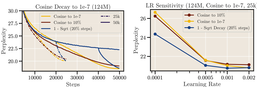
This figure compares the performance of cosine learning rate scheduling with a constant learning rate with cooldown. The left panel shows that the cooldown phase produces a sharp drop in loss, mirroring the behavior of cosine scheduling. The right panel shows that both methods have similar sensitivity to learning rate, although the constant + cooldown approach exhibits slightly lower sensitivity. The optimal learning rate for the constant + cooldown is also slightly lower than that for the cosine schedule.

This figure shows the final validation perplexity for different model sizes (33M, 53M, 60M, 93M, 124M, 151M, 210M, 360M parameters) across four different training methods: Cosine LR, Cooldown, SWA Cosine, and SWA Constant. The bar chart visually compares the performance of each method for each model size, allowing for a direct assessment of how different training schedules affect the final validation perplexity. This data supports the paper’s findings on the effectiveness of alternative training schedules compared to the traditional cosine learning rate schedule.

This figure compares the computational cost (in terms of FLOPs and GPU hours) of scaling experiments using the cosine schedule (Chinchilla’s approach) versus the proposed cooldown and SWA methods. The left panel shows the results of the authors’ experiments, demonstrating a significant reduction in both compute and GPU hours when using cooldown and SWA compared to the cosine schedule. The right panel shows a similar cost reduction for the Chinchilla experiments, highlighting the overall efficiency gains from using the alternative methods. The reduction in cost is more pronounced when more training runs are performed per model size, emphasizing the scalability and cost-effectiveness of the proposed approach.

This figure compares the computational cost of obtaining scaling laws using the cosine learning rate schedule (as in the Chinchilla paper) and the proposed cooldown schedule and stochastic weight averaging (SWA) techniques. The left panel shows the FLOPS and GPU hours used in the authors’ experiments across various model sizes, highlighting the significant reduction in computational resources achieved by the proposed methods. The right panel provides an estimation of the computational savings that would have been achieved in the Chinchilla experiments if a cooldown schedule was used instead of the cosine schedule.
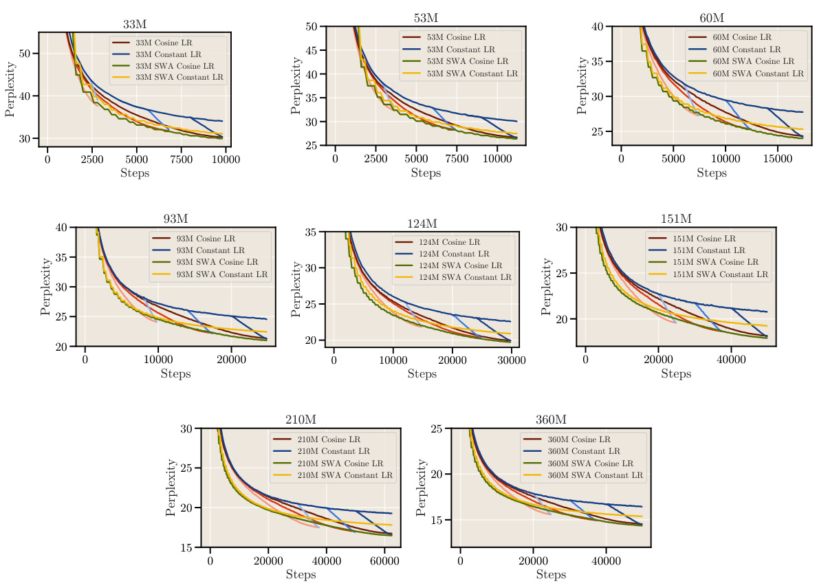
This figure shows the validation loss curves (perplexity) for all the models used in the scaling experiments described in Section 5 of the paper. The curves illustrate the training progress for different model sizes and configurations (Cosine LR, Constant LR, SWA Cosine LR, and SWA Constant LR) over a number of training steps. The visualization helps to compare the performance of different training schedules and the impact of Stochastic Weight Averaging (SWA) on the learning process.

This figure demonstrates the transferability of the findings from the SlimPajama dataset to the OpenWebText2 dataset. It shows that the consistent performance improvements observed with cooldown schedules and Stochastic Weight Averaging (SWA) on SlimPajama also hold true for OpenWebText2, reinforcing the robustness and generalizability of the proposed methods.

This figure compares the computational cost (in FLOPs and GPU hours) of scaling experiments using the proposed cooldown and SWA methods against the traditional Chinchilla method. It shows that the cooldown and SWA methods significantly reduce the computational resources required to obtain scaling laws, even more so when multiple experiments are run for each model size.
This figure compares the loss curves and learning rate sensitivity of two learning rate schedules: cosine annealing and constant learning rate with cooldown. The left panel shows that the cooldown phase in the constant learning rate schedule leads to a sharp decrease in loss, similar to the cosine annealing schedule. The right panel demonstrates that the optimal learning rate for both schedules is comparable, with the constant learning rate schedule showing slightly less sensitivity and the optimum learning rate being slightly lower than that for the cosine annealing schedule.
This figure shows the perplexity and learning rate curves for language models trained with cosine and constant learning rate schedules. It highlights that cosine schedules achieve optimal performance only when the training length perfectly matches the schedule cycle length. Stopping training early or continuing beyond the cycle leads to suboptimal results. This motivates the exploration of alternative training schedules that can produce good performance without this constraint.
More on tables

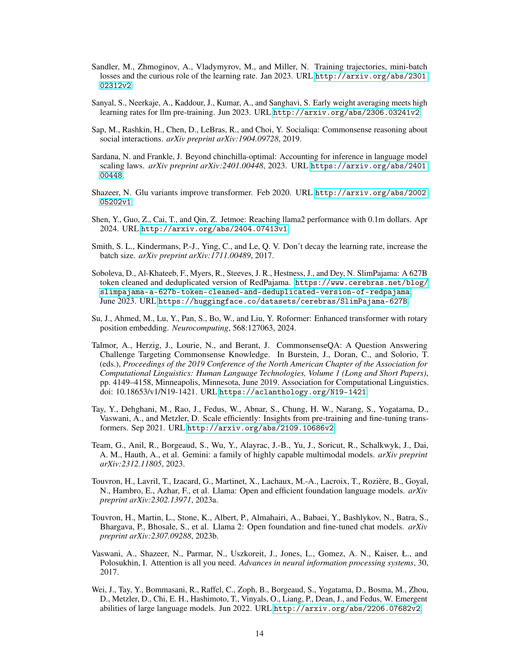
This table lists the configurations of various transformer models used in the scaling experiments. Each model is identified by its total number of parameters, and then various architectural hyperparameters are listed: The dimensionality of the model’s embedding, the number of layers, the feedforward network size, the key/value size, and the number of attention heads.
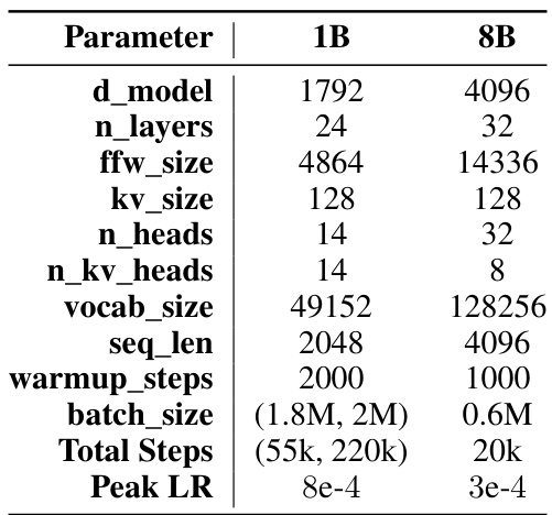
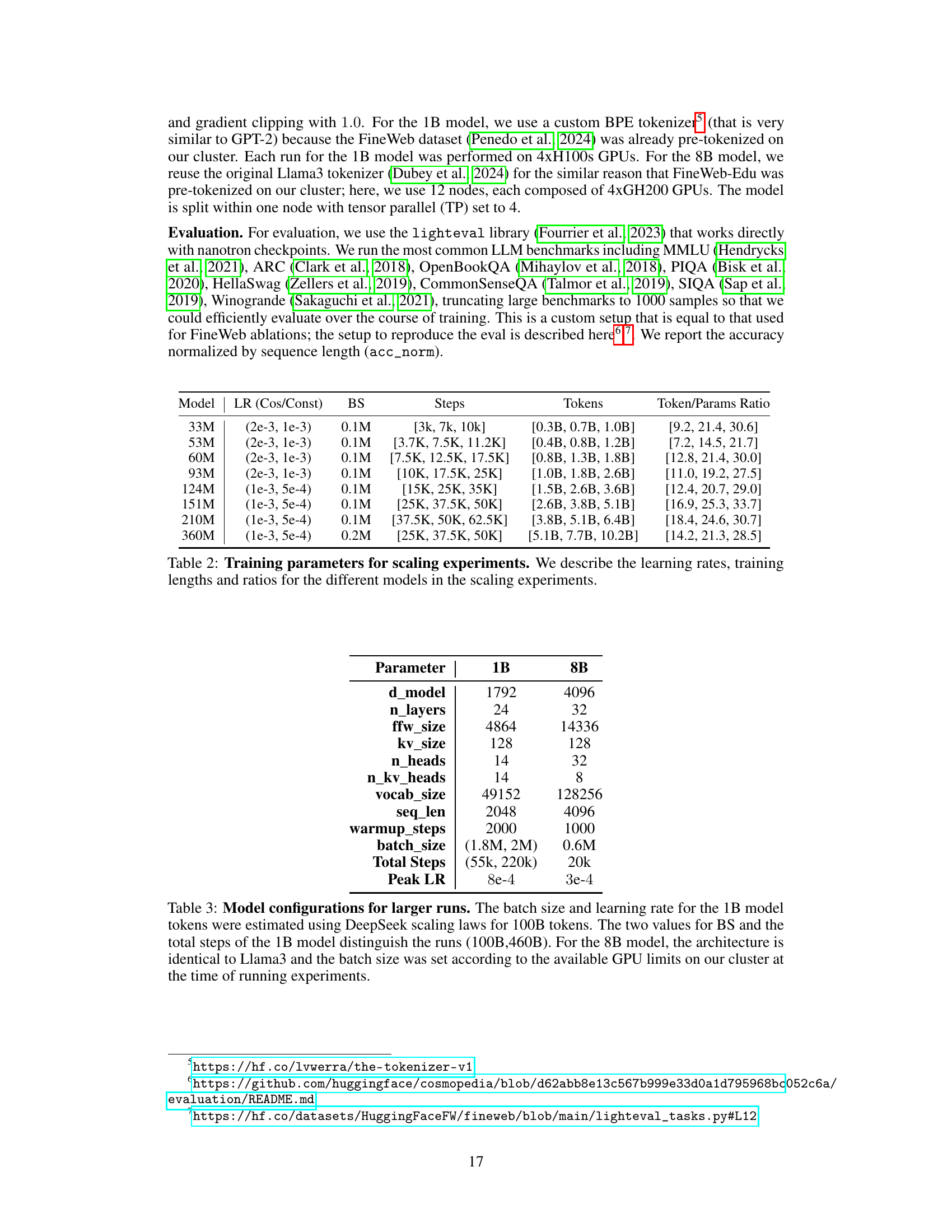
This table presents the hyperparameters used for training the 1B and 8B parameter models. Note that the batch size and learning rate for the 1B model were determined using DeepSeek scaling laws. The different values for batch size and total steps reflect experiments with different token counts (100B and 460B). The 8B model architecture follows that of Llama3, with the batch size adjusted to match the available GPU resources.
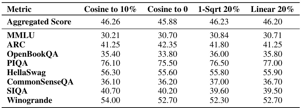
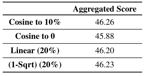
This table presents the final evaluation results obtained after training a 1B parameter model on 100B tokens. It compares the performance of four different learning rate schedules: cosine decay to 10% of the maximum learning rate, cosine decay to 0, a cooldown schedule using a 1-sqrt decay function (with 20% of the steps allocated to the cooldown), and a linear cooldown (also with 20% of steps). The metrics evaluated are an aggregated score and several individual benchmarks including MMLU, ARC, OpenBookQA, PIQA, HellaSwag, CommonSenseQA, SIQA, and Winogrande.

This table presents the final evaluation results obtained after training language models with 460B tokens using various cooldown schedules. It compares the aggregated scores and individual benchmark results (MMLU, ARC, OpenBookQA, PIQA, HellaSwag, CommonSenseQA, SIQA, Winogrande) for different cooldown lengths (5%, 10%, 20%) and a cosine schedule (decay to 0). The results show that while the performance of cosine and cooldown schedules are comparable, longer cooldown durations do not necessarily lead to better performance. This finding supports the proposed cooldown schedule as a practical alternative to the more computationally expensive cosine schedule.
Full paper#
