↗ OpenReview ↗ NeurIPS Proc. ↗ Chat
TL;DR#
Averaging probability distributions is crucial in many fields, but standard methods often fail to capture their geometric properties. Optimal Transport (OT) barycenters offer a mathematically grounded solution, but computing them, especially in the continuous setting, remains challenging. Existing continuous OT barycenter solvers often suffer from limitations such as restricting to specific cost functions or requiring non-trivial a priori selections, hindering their applicability to real-world scenarios. This paper addresses these challenges.
This work introduces a novel algorithm to approximate continuous EOT barycenters for arbitrary OT cost functions. It leverages the dual reformulation of the EOT problem and connects seamlessly with Energy-Based Models (EBMs). The method provides quality bounds, avoids complex optimization tricks, and is validated on low-dimensional and image-space setups, including non-Euclidean costs. The authors also demonstrate learning the barycenter on an image manifold generated by a pretrained GAN, showcasing its practical use and suggesting new directions for real-world applications. The method’s versatility and strong theoretical foundation make it a significant contribution to the field.
Key Takeaways#
Why does it matter?#
This paper is important because it presents a novel algorithm for efficiently computing continuous Entropic Optimal Transport (EOT) barycenters for various cost functions. This addresses a significant challenge in optimal transport, offering improvements over existing methods in terms of speed, applicability, and theoretical guarantees. It opens avenues for real-world applications in diverse fields dealing with probability distributions and provides strong theoretical backing for the method.
Visual Insights#

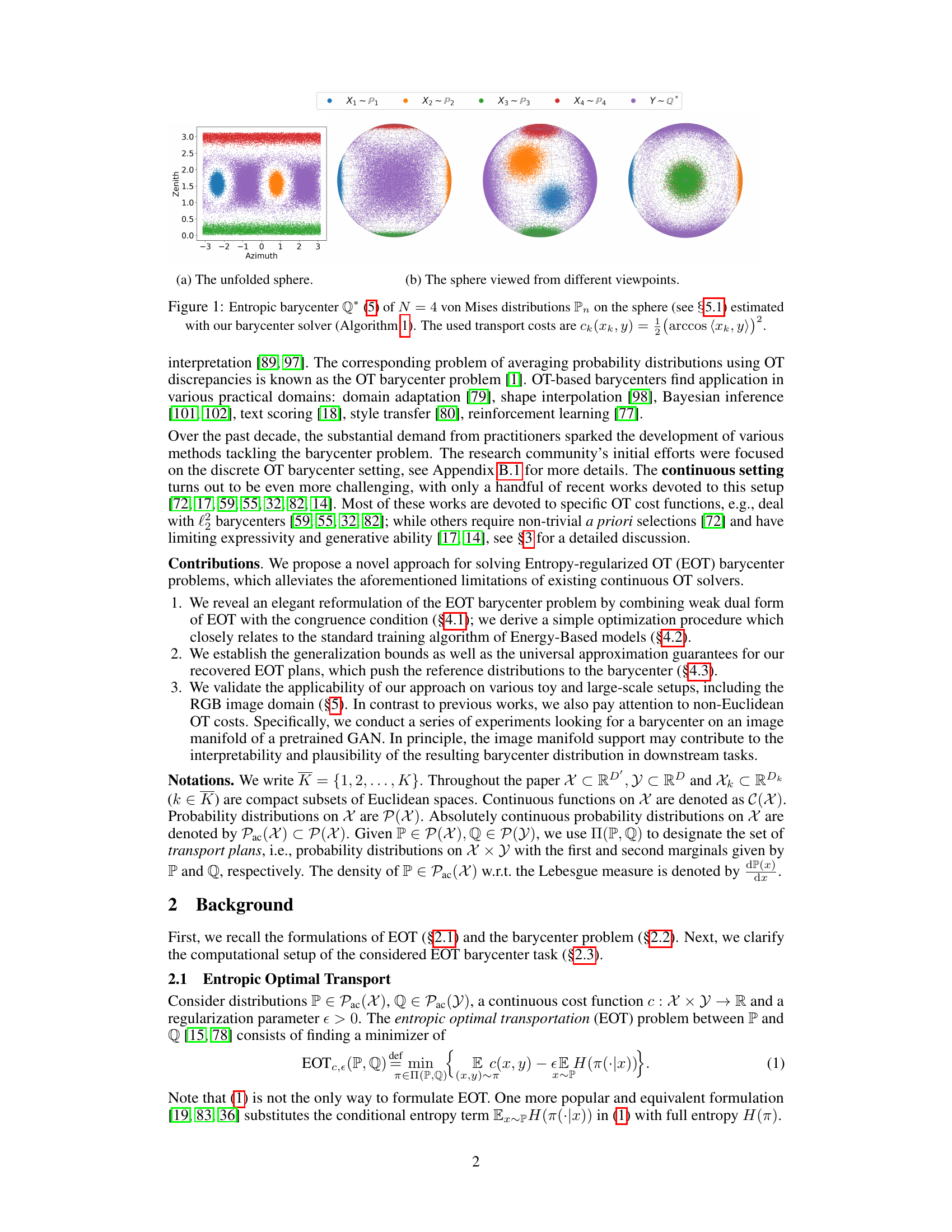
This figure visualizes the results of estimating the entropic barycenter of four von Mises distributions on a sphere using the proposed algorithm. The figure shows the unfolded sphere and three different viewpoints of the sphere with the four distributions and the estimated barycenter. The color-coding distinguishes the four distributions and the barycenter. The transport cost used is based on the squared arccosine distance between points on the sphere.
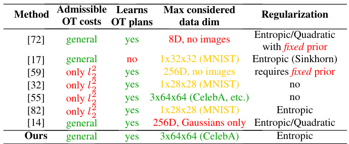
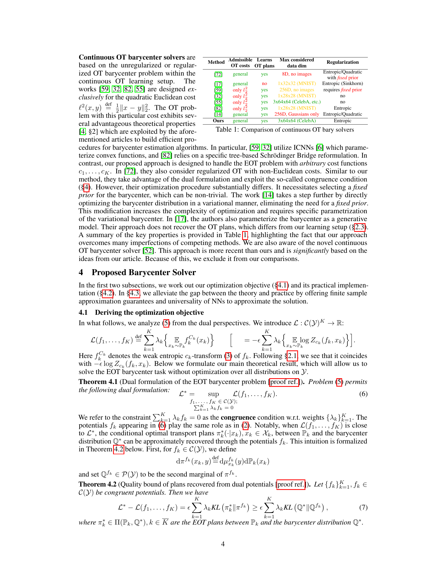
The table compares several continuous optimal transport (OT) barycenter solvers in terms of admissible OT cost functions, whether they learn OT plans, and the maximum data dimensionality they can handle. It also notes the type of regularization used. This allows for a comparison of the capabilities and limitations of various state-of-the-art approaches in the field.
In-depth insights#
EGB Barycenter Solver#
The Energy-Guided Barycenter (EGB) solver presents a novel approach to computing continuous Entropic Optimal Transport (EOT) barycenters. Its key innovation lies in leveraging the dual formulation of the EOT problem and connecting it to Energy-Based Models (EBMs). This allows the use of efficient EBM training algorithms, avoiding complex min-max or reinforcement learning techniques. The solver is shown to provide an intuitive optimization scheme, offers quality bounds for the recovered solutions, and seamlessly integrates with pretrained generative models for real-world applications. A significant advantage is its ability to handle arbitrary cost functions, expanding its applicability beyond traditional Euclidean distances. While the use of MCMC for sampling introduces computational costs, the approach enjoys both generalization bounds and universal approximation properties, ensuring robust and accurate results. Overall, the EGB solver provides a flexible and efficient way to approximate continuous EOT barycenters in diverse settings.
EOT Dual Reformulation#
Entropic Optimal Transport (EOT) dual reformulation offers a powerful alternative to the primal formulation for solving optimal transport problems. It leverages the concept of weak duality, providing a more computationally efficient approach by transforming the problem into a maximization of a dual objective function. This reformulation often involves the use of the weak entropic c-transform, simplifying the optimization process and avoiding some of the numerical challenges associated with the primal formulation. By focusing on the dual, the computational cost is often reduced, especially for high-dimensional problems, making it amenable to large-scale applications. Furthermore, it establishes a direct connection between optimal transport and energy-based models (EBMs). The EOT dual reformulation facilitates the application of well-established EBM techniques, such as stochastic gradient ascent and Markov chain Monte Carlo (MCMC) methods, significantly enhancing the practicality of EOT solutions. The inherent connection between EOT and EBMs highlights the potential synergy between optimal transport and deep learning frameworks, paving the way for innovative algorithms and applications in machine learning and various other fields.
Gen Bounds & Approx#
The heading ‘Gen Bounds & Approx’ likely refers to a section discussing generalization bounds and approximation guarantees within a machine learning context. This section would address the crucial question of how well a model trained on a finite dataset will perform on unseen data (generalization) and how accurately the model approximates the underlying theoretical concept it aims to model (approximation). Generalization bounds provide theoretical limits on the model’s performance on unseen data, offering insights into model complexity and data size needed for good generalization. Approximation guarantees, on the other hand, focus on the model’s ability to accurately learn the target function or distribution. This analysis would likely involve mathematical tools from statistical learning theory to quantify the approximation and generalization errors. The authors would likely present theorems and proofs establishing the bounds and guarantees, demonstrating that under certain conditions, the model’s errors can be controlled and reduced. The results are significant because they provide confidence in the model’s reliability and predictive capabilities. They would form a critical part of the paper, justifying the proposed model’s theoretical soundness and its potential practical success. The discussion might also include comparisons of the bounds and guarantees with existing methods, highlighting the advantages of the approach presented in the paper.
Manifold Barycenter#
The concept of a “Manifold Barycenter” extends the idea of averaging probability distributions beyond traditional vector spaces. Instead of calculating a simple mean, it leverages the geometry of a manifold, a curved space where the data resides. This is crucial when dealing with data points that aren’t easily represented by Euclidean coordinates—images, for example, are often better represented on a manifold. Finding the barycenter on a manifold involves searching for a point that minimizes the average distance to a set of distributions, accounting for the inherent curvature. The algorithm presented uses an energy-based model approach to estimate the barycenter, which offers advantages in terms of scalability and the ability to handle diverse cost functions. This method’s strength lies in its capacity to approximate the optimal transport plan between the source distributions and the barycenter, enabling better analysis of the relationships between the data. The use of a pre-trained generative model to define the manifold further enhances the method’s practical applicability, allowing for the exploration of non-Euclidean spaces and potentially improving interpretability. Overall, the manifold barycenter approach provides a more sophisticated and robust means of averaging probability distributions, especially relevant for complex, high-dimensional data.
Future Work & Limits#
Future research directions stemming from this work could explore several avenues. Extending the methodology to handle more general optimal transport (OT) cost functions beyond those considered is crucial for broader applicability. Investigating alternative optimization techniques to improve efficiency and scalability is also essential. The current reliance on Markov Chain Monte Carlo (MCMC) methods, while effective, can be computationally expensive; exploring alternative sampling strategies could significantly improve the algorithm’s performance. A detailed investigation of the effects of different regularization parameters on the accuracy and stability of the barycenter estimation is warranted. Finally, applying this energy-guided approach to higher dimensional data, such as high-resolution images or other complex data types, would help validate the model’s robustness and scalability. Addressing these limitations would significantly enhance the practical impact and utility of this novel barycenter estimation method.
More visual insights#
More on figures

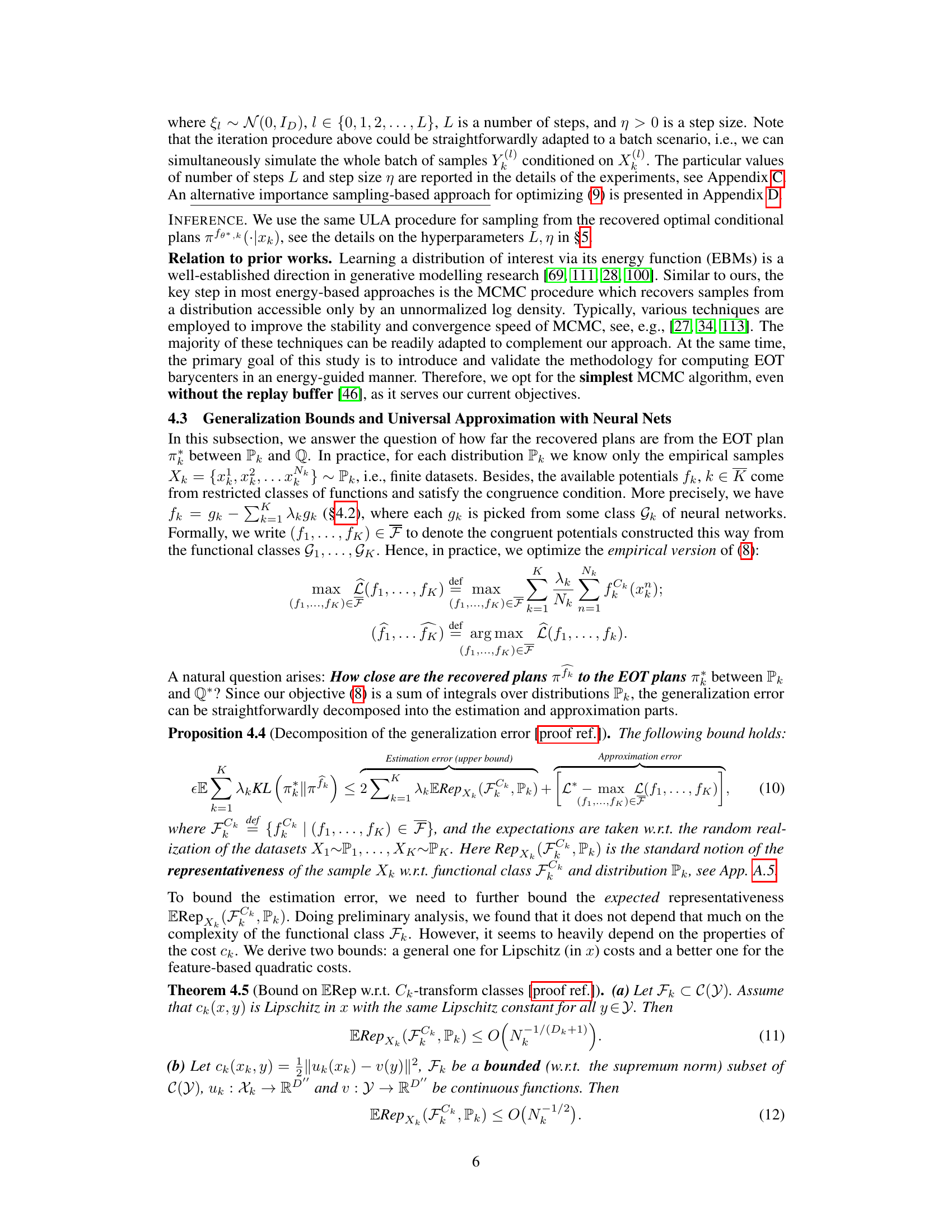
This figure shows a comparison of the true unregularized barycenter and the EOT barycenter computed by the proposed solver for a 2D twister example. The true barycenters were computed for both a twisted cost and the standard l² cost. The figure visualizes how the proposed method’s approximation of the barycenter compares to the ground truth barycenter in these two different cost function scenarios.
This figure visualizes the results of estimating an entropic barycenter of four von Mises distributions on a sphere using the proposed algorithm. Panel (a) shows the unfolded sphere. Panel (b) shows the sphere viewed from different angles, with each point representing a sample from one of the four von Mises distributions (P1-P4), and the barycenter (Q*). The color-coding helps distinguish the different distributions and the barycenter’s position relative to them. The squared arccosine of the angle between points is used as the transport cost.
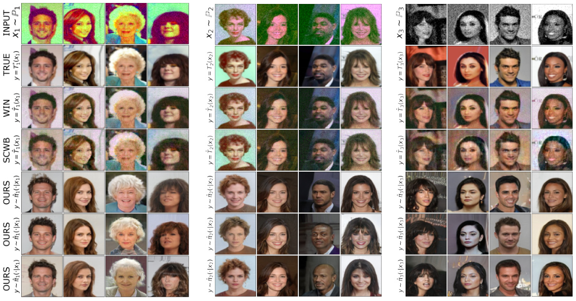
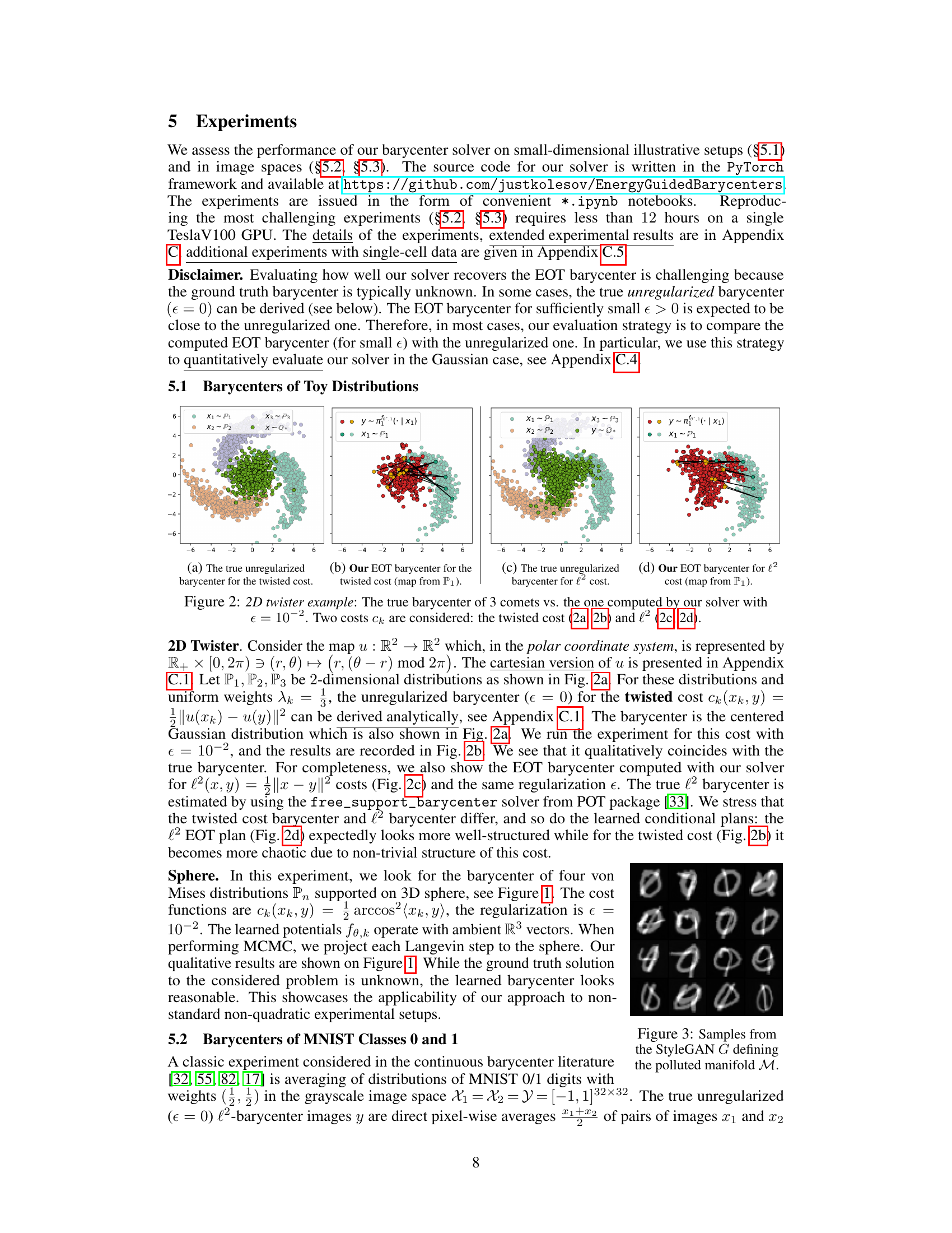
This figure compares the results of different barycenter solvers on the Ave, celeba! dataset. It shows the mappings from three different source distributions (P1, P2, P3) to the learned barycenter. The top row displays the input images from each distribution. The subsequent rows showcase the results produced by various solvers, including the ground truth, WIN, SCWB and the authors’ proposed method (OURS) with and without manifold constraints. The ground truth consists of clean celebrity faces, as referenced in the cited work [55, §5]. The figure visually demonstrates the effectiveness of the proposed method in generating more realistic and less noisy barycenter images compared to other state-of-the-art approaches, particularly when the manifold constraint is applied.

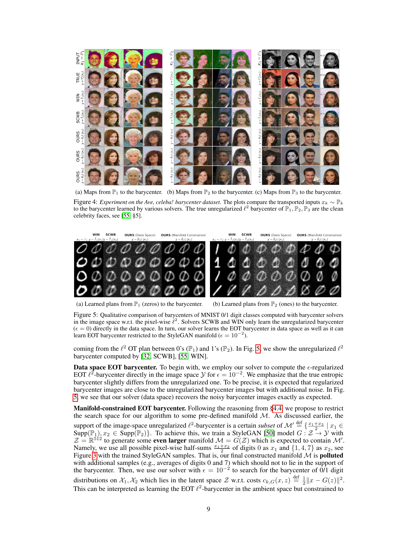
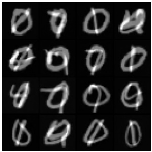
This figure compares the results of different barycenter solvers on MNIST 0 and 1 digit classes. It shows the learned transport maps from the input distributions (zeros and ones) to the barycenter. The comparison highlights the differences between solvers that operate directly in the image space versus those that utilize a StyleGAN manifold for learning the barycenter. The results showcase the ability of the proposed method to handle the e-regularized EOT barycenter problem and to leverage the pretrained StyleGAN generative model for generating a smoother, less noisy result.
This figure shows the results of estimating the entropic barycenter of four von Mises distributions on a sphere using the proposed barycenter solver. The barycenter Q* is visualized in panel (a) as an unfolded sphere, and in panel (b) from different viewpoints. The algorithm uses a specific cost function based on arccosine distance.
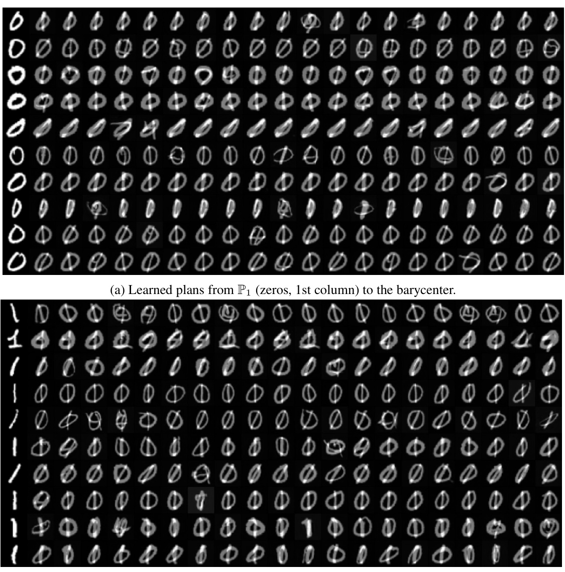
This figure shows additional examples of samples transported to the barycenter from the MNIST 0 and 1 digit classes. The images illustrate the results of applying the proposed EOT barycenter solver to these classes. The top panel shows the samples transported from the class 0 (zeros) and the bottom panel shows the samples transported from the class 1 (ones). Each column represents a different sample from the input distributions, and each row represents a different sample from the transported distribution.
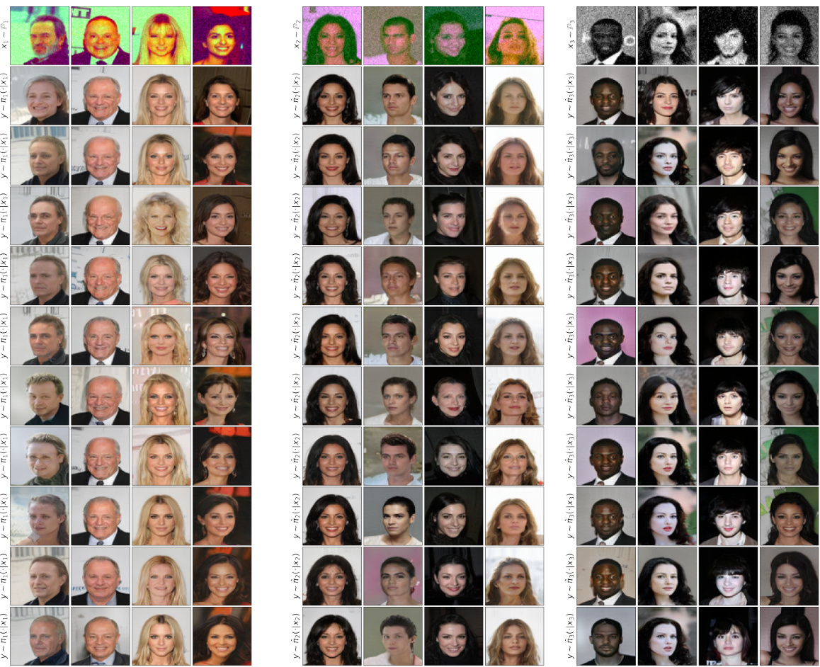
This figure compares the results of different continuous optimal transport (OT) barycenter solvers on the Ave, celeba! dataset. It shows how different methods transport samples from three input distributions (P1, P2, P3) to the estimated barycenter. The true barycenter, known beforehand for this dataset, consists of clean celebrity images. The figure highlights the visual differences in the mappings produced by various solvers, illustrating the effect of the chosen method on the quality and characteristics of the resulting barycenter.

This figure visualizes the results of estimating the entropic barycenter of four von Mises distributions on a sphere using the proposed algorithm. Panel (a) shows the unfolded sphere for better visualization. Panel (b) displays the sphere from various viewpoints, highlighting the four von Mises distributions (in different colors) and the estimated barycenter (in purple). The algorithm uses a cost function based on the squared arccosine distance between points on the sphere.

This figure compares the results of different optimal transport (OT) barycenter solvers on the Ave, celeba! dataset. The dataset consists of three sets of degraded celebrity faces (P1, P2, P3). The goal is to find a barycenter, a representative average face. The figure shows how input faces from each set (xk ~ Pk) are transformed (mapped) to the barycenter by each solver. The ’true’ unregularized l² barycenter (the clean celebrity faces) is used as a reference for comparison, allowing for a visual assessment of each solver’s accuracy.
This figure visualizes the result of estimating the entropic barycenter of four von Mises distributions on a sphere using the proposed algorithm. Panel (a) shows the unfolded sphere, while panel (b) presents different viewpoints of the sphere with the four distributions and the estimated barycenter highlighted. The cost function used is based on the arccosine distance between points on the sphere.

This figure shows a comparison of the true unregularized barycenter and the EOT barycenter computed using the proposed method for a 2D twister example. The example involves three comet-shaped distributions. Two different cost functions are used for comparison: a twisted cost and the standard Euclidean l2 cost. The plots visualize the distributions and their corresponding barycenters, illustrating the differences obtained when using different cost functions and regularization.
More on tables

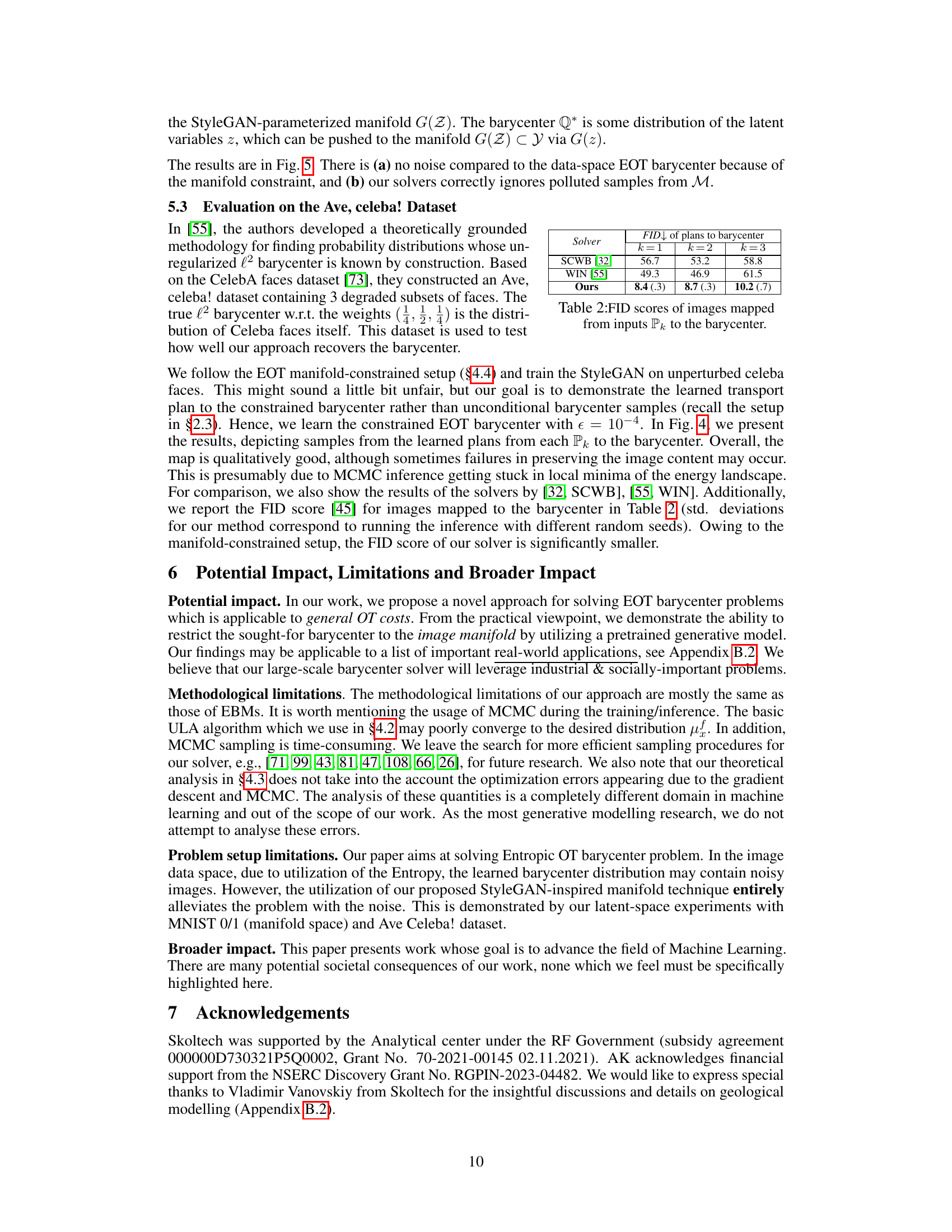
This table compares the Fréchet Inception Distance (FID) scores achieved by different continuous optimal transport (OT) barycenter solvers. Lower FID scores indicate better quality of the generated images. The table shows the FID scores for three different subsets of data (k=1, k=2, k=3) and compares the performance of the proposed method (‘Ours’) to two existing methods: SCWB [32] and WIN [55]. The results demonstrate that the proposed method significantly outperforms the baselines in terms of image quality.
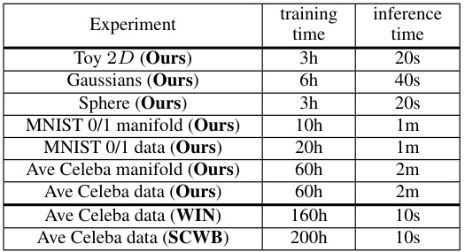
This table compares different continuous optimal transport (OT) barycenter solvers in terms of the types of OT cost functions they support, whether they learn OT plans or just the barycenter, the type of regularization used (if any), and the maximum dimensionality of the data they can handle. It highlights that many existing solvers are limited to specific cost functions or require pre-selected priors, while the proposed method addresses these limitations.

The table compares different continuous optimal transport (OT) barycenter solvers. It lists the admissible OT costs (cost functions), whether they learn the OT plans directly, the maximum considered data dimensionality and the type of regularization used (Entropic or Quadratic). The table highlights the differences in the capabilities and limitations of the existing methods.
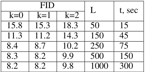
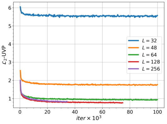
This table shows how the running time of the ULA (unadjusted Langevin algorithm) during inference changes with the number of Langevin steps (L) used. It also demonstrates the trade-off between the number of steps and the quality of the resulting images in the Ave, Celeba! dataset when using the manifold-constrained setting. As the number of steps increases, so does the quality (FID score decreases), but also the time required for inference increases.
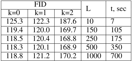
This table shows the relationship between the number of Langevin steps (L) used during the inference phase of the EOT barycenter calculation and the resulting FID scores and computation time. It demonstrates the trade-off between computational cost (time) and the quality (FID) of the generated images in the Ave, Celeba! dataset. Different values of L are tested and their impact on FID (for different components k=0,1,2) and the time in seconds are reported.

This table presents the L2-UVP (unexplained variance percentage) results for the proposed method and compares them to the WIN method’s results. L2-UVP is a metric used to evaluate the quality of learned optimal transport maps. The table shows the results for different dimensions (D) and regularization strengths (ε). Lower L2-UVP values indicate better performance.

This table presents the energy distance results for different solvers on the MSCI dataset. The energy distance is a measure of the dissimilarity between probability distributions. The results are averaged over two setups and five random seeds, with 95% confidence intervals provided. The best performing solver for each dimension is highlighted in bold.

This table shows the effect of batch size on the performance of the proposed EOT barycenter solver when computing barycenters of Gaussian distributions. The results are measured by the L2-UVP metric, which assesses the difference between the obtained and the true optimal transport plan. Lower L2-UVP values indicate better performance. The table presents results for two different scenarios: (D, ε) = (2, 0.1) and (D, ε) = (16, 0.01), where D is the dimension of the data and ε is the regularization parameter.
Full paper#
