Schrodinger Bridge Flow for Unpaired Data Translation

1F32iCJFfa

Valentin De Bortoli et el.

TL;DR
#

Many machine learning tasks involve mapping one probability distribution to another. Optimal Transport (OT) provides a theoretical framework for this, but traditional OT methods are computationally expensive, especially for high-dimensional data. Existing approximation methods, while offering better computational efficiency, still suffer from limitations; they often fail to accurately approximate OT and may introduce significant errors. This necessitates the development of more efficient and accurate algorithms.

Key Takeaways
#

Why does it matter?
#

This paper is crucial for researchers working on unpaired data translation and generative modeling. It offers a novel, efficient algorithm for a fundamental problem in machine learning, bridging the gap between theoretical optimality and practical applicability. The Schrödinger Bridge Flow offers a new avenue for research, potentially impacting various fields using optimal transport, such as image-to-image translation and transfer learning.

Visual Insights
#

This figure illustrates the Schrödinger Bridge Flow (SBF) and compares it to Iterative Markovian Fitting (IMF). It shows how the SBF iteratively refines a path measure (represented by the orange curve), starting from an initial distribution (P0) until it converges to the Schrödinger Bridge (P*). The figure also highlights that Markov processes (M) and those in the reciprocal class of Q (R(Q)) are involved in the iterative refinement.

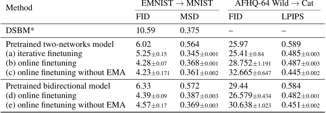
This table presents the results of image translation experiments using different methods: DSBM (from Shi et al., 2023), and the proposed a-DSBM method with different model architectures (two-networks vs. bidirectional) and finetuning approaches (iterative vs. online, with/without EMA). Results are shown for FID (Fréchet Inception Distance) and MSD (Mean Squared Distance) metrics on the EMNIST to MNIST task, and FID and LPIPS (Learned Perceptual Image Patch Similarity) metrics on the AFHQ-64 Wild to Cat task. Error bars (standard deviations) are included for the a-DSBM results.

In-depth insights
#

Schrödinger Bridge Flow
#

The concept of “Schr C366dinger Bridge Flow” presents a novel algorithm for efficiently computing the Schr C366dinger Bridge, a dynamic, entropy-regularized optimal transport method. It avoids the computationally expensive training of multiple diffusion models at each iteration, unlike previous methods. Instead, it leverages a discretization of a flow of path measures, hence the name, directly targeting the Schr C366dinger Bridge as a fixed point. This approach offers significant advantages in high-dimensional data scenarios, where existing techniques often struggle due to computational complexity and mini-batch errors. The core innovation lies in its iterative refinement process which directly refines a flow of path measures, converging to the Schr C366dinger Bridge without requiring repeated training of complex models. This leads to improved efficiency and accuracy, particularly in challenging unpaired data translation tasks where a direct map between distributions is sought. The algorithm also provides flexibility through a tunable parameter, controlling the convergence speed and potentially offering online adaptability. The resulting method demonstrates promising results in various unpaired data translation experiments.

Unpaired Data Xlation
#

Unpaired data translation, a significant challenge in machine learning, focuses on mapping data distributions without requiring paired examples. This poses difficulties for traditional methods reliant on correspondence between source and target data. The paper explores novel approaches to address this by leveraging optimal transport (OT) techniques and diffusion models. The core idea is to find a transformation that optimally maps one distribution to another, addressing limitations of existing methods like CycleGAN and Bridge Matching which don’t exactly approximate OT maps. The proposed technique offers improved accuracy and efficiency by directly computing the Schrödinger Bridge, a dynamic entropy-regularized version of OT, without the need for iterative training of multiple diffusion models. This is achieved via a novel algorithm called Schrödinger Bridge Flow, resulting in significant speedups during data translation. The algorithm’s efficiency and scalability are demonstrated through experiments on several unpaired image translation tasks, suggesting significant advantages in handling high-dimensional data.

a-DSBM Algorithm
#

The a-DSBM algorithm presents a novel approach to unpaired data translation by efficiently computing the Schrödinger Bridge. Unlike previous methods, it avoids training multiple DDM-like models at each iteration, significantly reducing computational cost and complexity. The core innovation lies in its formulation as a discretisation of a flow of path measures, thereby eliminating the need for iterative Markovian fitting. This flow’s only stationary point is the Schrödinger Bridge, ensuring convergence to the optimal solution. The algorithm’s efficiency is demonstrated through its online nature and the use of a single neural network, making it a significant advancement for high-dimensional data translation tasks. While offering substantial improvements, future work could explore further optimization techniques and address potential error accumulation in very high dimensions to enhance robustness and scalability.

Online vs. Iterative
#

The core of the “Online vs. Iterative” comparison lies in the method of updating model parameters. Iterative approaches, like traditional DSBM, involve complete training cycles for each model update, resulting in high computational costs but potentially more stable convergence. In contrast, the online approach updates the model incrementally, using each data sample only once, significantly reducing computation time. However, online learning might sacrifice stability for speed, potentially leading to suboptimal solutions or slower convergence to the true Schrödinger Bridge. The paper highlights a trade-off: iterative methods provide potentially superior convergence but at higher computational expense, whereas online methods are significantly faster but the price is potential instability. The choice between online and iterative approaches is highly dependent on the dataset size, computational resources, and desired accuracy. The introduction of α-DSBM aims to offer a spectrum, enabling a balance to be struck between the two extremes.

Future Research
#

Future research directions stemming from this work on Schrödinger Bridge Flow for unpaired data translation could explore several key areas. Improving the efficiency and scalability of the algorithm for even larger datasets and higher dimensions is crucial. This might involve exploring more efficient numerical methods, or approximations that reduce computational complexity while retaining accuracy. Another promising avenue is to investigate alternative parameterizations of the vector fields, potentially using more efficient architectures or employing different techniques like normalizing flows. Extending the method to more complex data modalities beyond images is important, such as time series or point clouds. Finally, a thorough investigation into the algorithm’s theoretical properties, including convergence rates and stability under different conditions, would be valuable. A particular focus could be placed on understanding the relationship between the algorithm’s hyperparameters (particularly the entropic regularization) and the resulting transport maps. Addressing the issue of sampling-free methodologies to remove the reliance on iterative sampling remains a significant challenge but a critical area for future development.

More visual insights
#

More on figures

This figure shows the evolution of the covariance matrix during the finetuning stage of the α-DSBM and DSBM algorithms. It compares the performance of online α-DSBM against iterative DSBM, highlighting the faster convergence of α-DSBM. Both scalar and full covariance matrices are considered, illustrating the robustness of the α-DSBM approach.

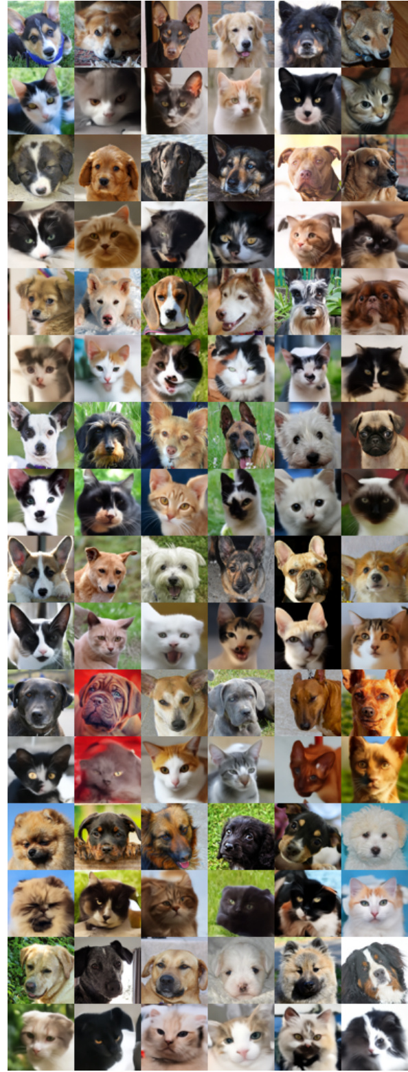
This figure shows the impact of the hyperparameter epsilon (ε) on the performance of the model for two different tasks: EMNIST to MNIST translation and AFHQ-64 image generation. The left panel presents FID and MSD scores before and after finetuning for various values of ε, illustrating that an optimal ε value exists. The right panel displays generated AFHQ-64 samples (64x64 resolution animal face images) after finetuning, showcasing the quality of the generated samples as affected by the choice of ε. Appendix K provides additional results.

This figure shows the results of online DSBM applied to the AFHQ 256x256 dataset. The top row displays the initial samples from the Cat and Wild domains before the translation process. The bottom row shows the results after the translation, which is achieved using online DSBM. This demonstrates the model’s ability to transfer images between these two domains using online DSBM.

This figure shows the results of EMNIST to MNIST image translation experiments. The left panel shows FID and MSD scores before and after finetuning the model with different values of epsilon (noise level), illustrating the impact of epsilon on the translation performance. The right panel displays example images generated by a bidirectional model after finetuning, showcasing the model’s ability to generate high-quality images after finetuning.

This figure illustrates the Schrödinger Bridge flow and compares it with Iterative Markovian Fitting (IMF). It highlights that the Schrödinger Bridge (SB) is the only fixed point of the flow, and under certain assumptions, it’s also a limit point of IMF. The figure also depicts the relationship between Markov processes (M), reciprocal classes of Q (R(Q)), and the SB (P*).

This figure illustrates the Schrödinger Bridge flow and how it compares to the Iterative Markovian Fitting (IMF) method. The Schrödinger Bridge (SB) is represented as the only fixed point of the flow, highlighting its unique role in the mass transport problem. The illustration shows how the iterative process of the IMF method converges towards this SB point.

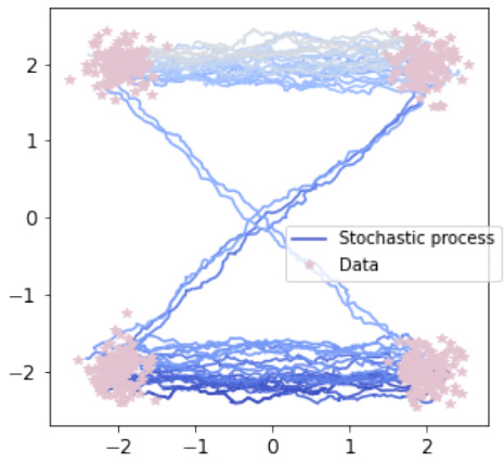
This figure illustrates the Schrödinger Bridge flow (SB Flow) and its comparison with the Iterative Markovian Fitting (IMF) method. The SB flow is a continuous process represented by curves converging towards the Schrödinger Bridge (P*). The IMF method is a discrete version of this process which is represented by a sequence of points approximating the SB. The key idea is that the SB is the only fixed point in the SB Flow, highlighting its unique property as a Markov process with prescribed marginals at the endpoints that belongs to the reciprocal class of the Brownian motion. The a-IMF procedure, a discretised version of SB flow, is also illustrated as it converges to SB for any α ∈ (0, 1], further highlighting the relationship between these procedures.

The figure shows the evolution of covariance matrices during training for different methods: online α-DSBM, iterative DSBM, and baseline bridge matching. It demonstrates how the online method converges faster and more efficiently toward the true covariance compared to iterative approaches, with varying frequencies of alternating forward and backward updates. The left panel shows results for a Gaussian distribution with a scalar covariance matrix; while the right panel illustrates results for a Gaussian distribution with a full covariance matrix.

This figure shows the evolution of the covariance matrix during the finetuning stage of the algorithm for both online and iterative versions, comparing α-DSBM against base and DSBM. It uses two Gaussian distributions with different covariance structures (scalar and full) to illustrate the convergence towards the true covariance matrix (optimum). The plots illustrate that α-DSBM converges faster to the true covariance than the iterative DSBM method.

This figure shows the evolution of covariance matrices during the training process of three different methods: the baseline bridge matching, the online α-DSBM, and the iterative DSBM. It demonstrates how quickly each method converges to the true covariance matrix, comparing different update frequencies for iterative DSBM. The left panel uses a simple Gaussian distribution with a scalar covariance matrix, and the right panel employs a Gaussian distribution with a full covariance matrix.

This figure shows the evolution of covariance matrices during the training process of different models: online α-DSBM, iterative DSBM, and a basic bridge matching model. The training starts after an initial 10,000 steps of training a bridge matching model. The left panel shows results for a Gaussian distribution with a scalar covariance matrix while the right panel shows results for a Gaussian distribution with a full covariance matrix. The plots show that the online α-DSBM method converges to the true covariance faster than the iterative DSBM method. The figure also illustrates the performance comparison between different variants of the methods.

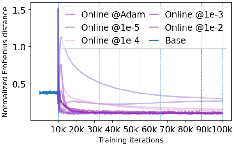
This figure shows the evolution of the covariance matrix during the training process of different methods: online α-DSBM, iterative DSBM, and the baseline bridge matching. The left panel displays results for a Gaussian distribution with a scalar covariance matrix, while the right panel shows results for a Gaussian distribution with a full covariance matrix. The plots illustrate how quickly each method converges to the true covariance, demonstrating the superior performance of the online α-DSBM approach.

This figure shows the evolution of the covariance matrix during the training process of different algorithms for unpaired data translation. The plot compares three methods: a baseline bridge matching, a novel online approach (α-DSBM), and the iterative DSBM. Both left and right panels show results for Gaussian distributions (scalar and full covariance, respectively). The key takeaway is that the online α-DSBM method converges faster to the true covariance than the iterative DSBM.

This figure shows the evolution of the covariance matrices during the training process for both iterative and online DSBM. The iterative method alternates between forward and backward updates at different frequencies (1k, 2.5k, and 5k steps), while the online method updates continuously. The plot compares the Frobenius norm between the estimated and true covariance matrices for the models. A Gaussian distribution with a scalar and full covariance matrix is used.

This figure shows the evolution of covariance matrices during training, comparing three different methods: online α-DSBM, iterative DSBM, and a baseline bridge matching method. The left panel shows results for a Gaussian distribution with a scalar covariance matrix, while the right panel shows results for a Gaussian distribution with a full covariance matrix. The results demonstrate that online α-DSBM converges to the true covariance faster than iterative DSBM, highlighting its efficiency. Different update frequencies are shown for the iterative DSBM to illustrate its behaviour as it approaches the online strategy.

This figure shows the evolution of the covariance matrix during the finetuning phase of the online and iterative versions of DSBM, comparing them with a base bridge matching model. The left panel shows results for a Gaussian distribution with a scalar covariance matrix, while the right panel shows results for a Gaussian distribution with a full covariance matrix. The plots illustrate how quickly the algorithms converge to the true covariance matrix and highlight the superior performance of the online α-DSBM method.

This figure shows the MNIST samples generated from EMNIST letter inputs by the base and fine-tuned models at different noise levels (ε). Low ε values produce poor sample quality, while high ε values lead to misalignment and blurriness. The fine-tuned model improves the quality, but still suffers from these issues at extreme ε values.

This figure shows the MNIST samples generated by the base and finetuned models with different noise levels (epsilon). The results show that very low noise levels lead to poor sample quality, which finetuning cannot fix, and excessively high noise levels lead to poor alignment and blurriness.

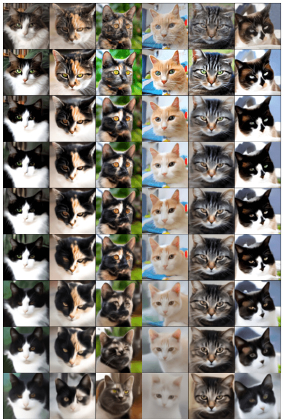
This figure shows the results of a Wild to Cat image translation experiment using a bidirectional model with online finetuning and different values of √e. The top row shows the initial samples. Subsequent rows show the results with different noise levels (√e). The results demonstrate a trade-off between sample quality and alignment. Low √e values result in poor sample quality, while excessively high √e values hinder the transfer of information and produce blurry, misaligned results.

The figure shows the evolution of the covariance matrix during the finetuning stage of the proposed a-DSBM algorithm compared to the original DSBM algorithm and the base bridge-matching model. Both online and iterative finetuning approaches are shown for two types of Gaussian distributions: one with a scalar covariance matrix, and another with a full covariance matrix. The plot displays how quickly each method converges to the optimal covariance matrix (indicated as ‘Optimum’). The results demonstrate that the online α-DSBM approach achieves faster convergence than the iterative DSBM, and that α-DSBM’s performance closely matches DSBM when the update frequency is high.

This figure shows the evolution of covariance matrices during the finetuning process of the DSBM model. Two different scenarios are shown: one using a scalar covariance matrix and another with a full covariance matrix. Three methods are compared: the baseline bridge matching, the online α-DSBM, and the iterative DSBM (with varying update frequencies). The normFrob metric measures the difference between the true covariance (C*) and the estimates from each method. The left panel shows results for a scalar covariance matrix, and the right panel for a full covariance matrix.

This figure shows the evolution of covariance matrices during training in different settings. It compares the convergence speed of three methods: a standard baseline (Bridge Matching), the proposed α-DSBM (online) method, and a more traditional iterative DSBM approach. Two scenarios are displayed: one with a simple scalar covariance matrix and one with a full covariance matrix. The plots demonstrate the faster convergence of the online a-DSBM compared to iterative DSBM, with the a-DSBM closely approximating the true covariance (optimum).

This figure displays the evolution of the covariance matrix during the finetuning phase of both online and iterative versions of the DSBM algorithm. Two different Gaussian settings are shown (scalar and full covariance). The graphs plot the Frobenius norm of the difference between the true covariance and the estimated covariance over training iterations, illustrating the convergence speed of the different methods. The iterative DSBM shows faster convergence as the frequency of switching between forward and backward updates increases, finally approaching the performance of the online α-DSBM.

This figure displays the evolution of covariance matrices during the finetuning stage of the DSBM algorithm. It compares three different approaches: online α-DSBM, iterative DSBM with varying update frequencies (1K, 2.5K, and 5K steps), and a baseline bridge matching model. The plots show that the online α-DSBM converges faster to the true covariance than the iterative DSBM approaches, and that both outperform the baseline. Two scenarios are shown: one with a scalar covariance matrix and one with a full covariance matrix, demonstrating the algorithm’s performance across different levels of complexity.

This figure shows the evolution of the covariance matrix during the training process for different methods: online α-DSBM, iterative DSBM, and base bridge matching. The left panel shows results for a Gaussian distribution with a scalar covariance matrix, while the right panel shows results for a Gaussian distribution with a full covariance matrix. The plots demonstrate how the covariance matrix changes during training and how quickly each method converges to the true value. The figure highlights the superiority of online α-DSBM over iterative DSBM in this task.

This figure shows the evolution of the covariance matrix during the finetuning process of the DSBM model, comparing three different approaches: online α-DSBM, iterative DSBM, and base bridge matching. It demonstrates that online α-DSBM converges to the true covariance faster than the other methods, especially for the more complex case of a full covariance matrix. The plots visualize the Frobenius norm difference between the estimated and actual covariance matrices over training iterations.

This figure shows the results of transferring images from the Wild domain to the Cat domain using a bidirectional model with different noise levels (√ε). The left column shows the results before finetuning and the right column shows the results after finetuning. It demonstrates that lower values of √ε result in poor image quality, while high values of √ε lead to blurry images and misalignment. A good √ε balances image quality and alignment.

The figure shows the evolution of the covariance matrix during the finetuning of the forward and backward networks in online and iterative DSBM. It compares the performance of three methods: a baseline bridge matching model, an online α-DSBM, and an iterative DSBM with varying frequencies of alternating between forward and backward updates. The results are presented for two scenarios: a Gaussian distribution with a scalar covariance matrix and a Gaussian distribution with a full covariance matrix. The plots display the Frobenius norm between the true covariance matrix and the estimated covariance matrix over training iterations. The online α-DSBM converges significantly faster than the iterative DSBM.

This figure shows the evolution of the covariance matrix during the finetuning of the DSBM model using three different approaches: online, iterative, and base. The plots show that the online α-DSBM algorithm is faster to converge and provide an accurate estimation of the covariance compared to iterative DSBM and base Bridge Matching.

This figure shows the evolution of covariance matrices during training for different methods: online and iterative DSBM, and a baseline bridge matching model. Two scenarios are presented, one with a scalar covariance matrix and another with a full covariance matrix. The plots illustrate the convergence speed and accuracy of the different algorithms toward the true covariance matrix (optimum).

This figure shows the evolution of covariance matrices during the training process for three different methods: online DSBM, iterative DSBM, and bridge matching. The results are presented for two different types of Gaussian distributions: one with a scalar covariance matrix and one with a full covariance matrix. The plots illustrate the convergence of the methods towards the true covariance matrix, with online DSBM showing faster convergence compared to iterative DSBM and bridge matching.

TL;DR#

Key Takeaways#

Why does it matter?#

Visual Insights#

In-depth insights#

Schrödinger Bridge Flow#

Unpaired Data Xlation#

a-DSBM Algorithm#

Online vs. Iterative#

Future Research#

More visual insights#

Full paper#