↗ OpenReview ↗ NeurIPS Proc. ↗ Chat
TL;DR#
Current methods for representing procedural activities often rely on hand-crafted procedures or complex graph mining techniques. These methods are not readily incorporated into neural architectures and may struggle with real-world video data which contains noise and inconsistencies. Furthermore, accurately detecting mistakes in complex procedures remains a challenge for AI systems.
This research introduces a novel, differentiable loss function (TGML) for learning task graphs directly from video. Two learning approaches are proposed: direct optimization (DO) of the graph’s adjacency matrix and a feature-based task graph transformer (TGT). Experiments demonstrate that the proposed method surpasses existing approaches in accuracy, significantly improving the prediction of task graphs and boosting online mistake detection. This is particularly impactful in areas such as instructional videos and egocentric activity analysis.
Key Takeaways#
Why does it matter?#
This paper is crucial for researchers in procedural activity understanding and computer vision due to its novel approach to learning task graphs directly from video data. The proposed method significantly improves online mistake detection in procedural videos and offers a novel differentiable loss function that can easily be integrated into other neural architectures. This opens new avenues for developing more robust and intelligent AI agents able to assist humans in performing complex tasks. The work’s focus on egocentric videos and online mistake detection aligns perfectly with current research trends in human-computer interaction and artificial intelligence.
Visual Insights#

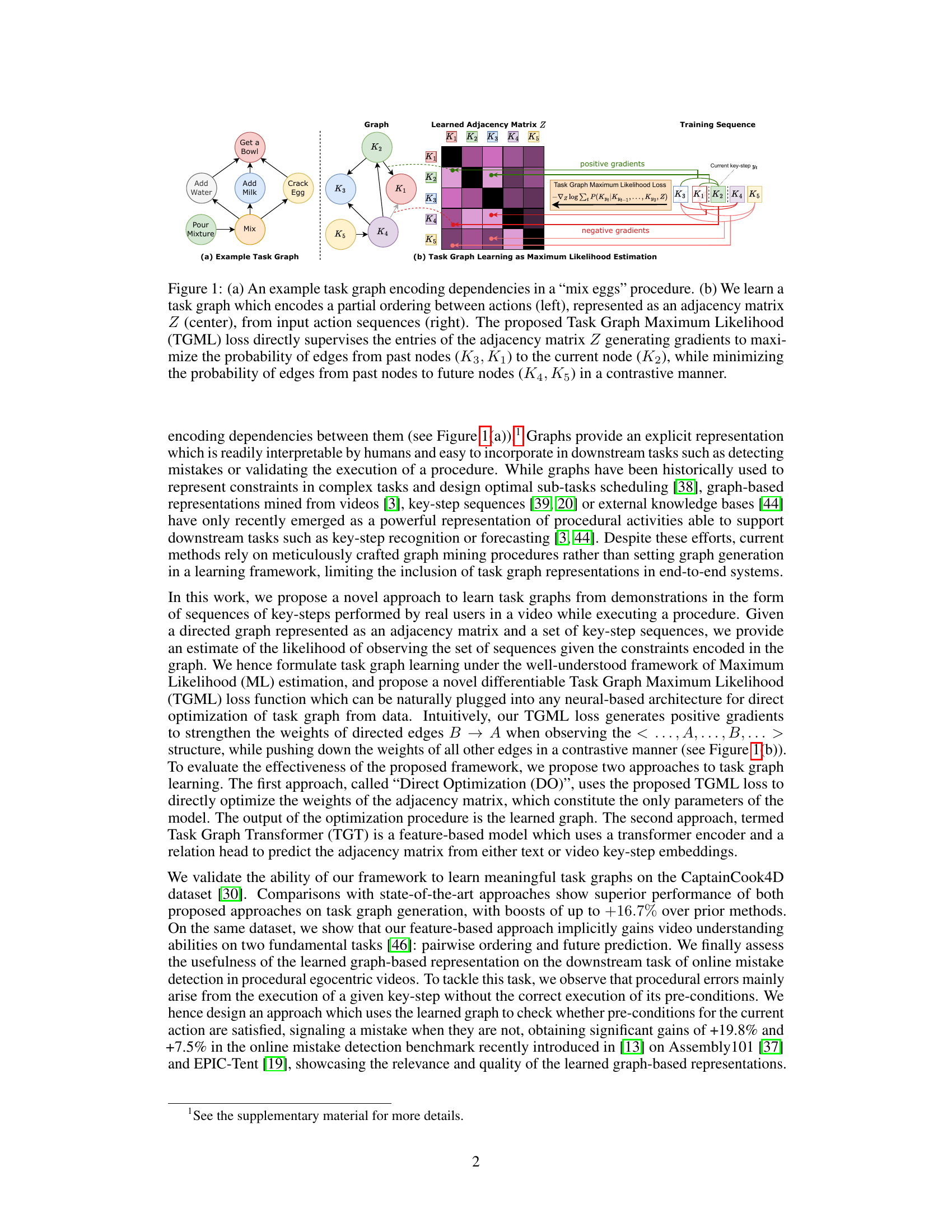
This figure illustrates the task graph learning process. (a) shows an example task graph representing a simple procedure. (b) details how the proposed Task Graph Maximum Likelihood (TGML) loss function learns the task graph from action sequences. The TGML loss function optimizes the weights of the adjacency matrix to accurately reflect the dependencies between actions by maximizing the likelihood of edges from previous actions to the current one and minimizing the likelihood of edges connecting previous actions to future ones.
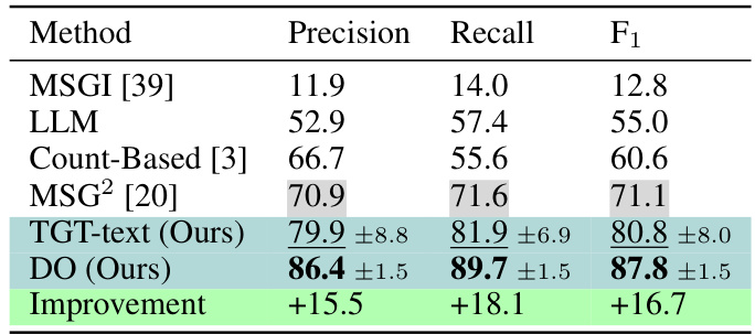
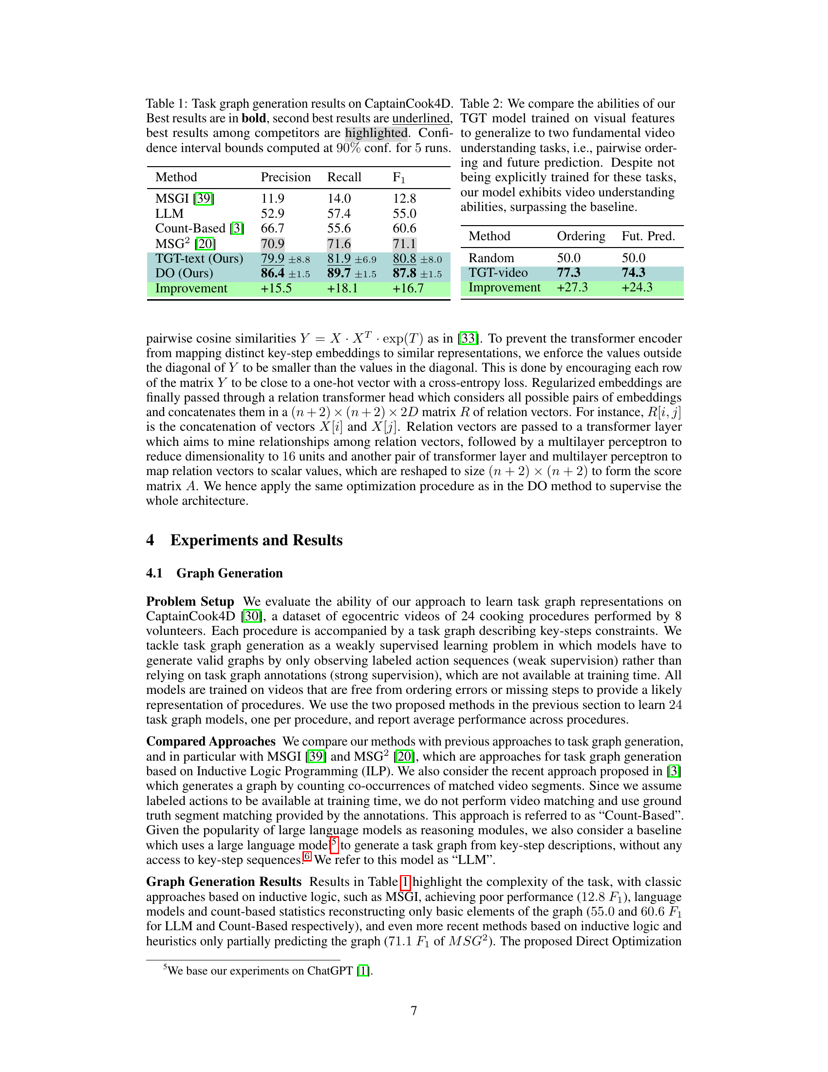
This table presents the performance of different methods for task graph generation on the CaptainCook4D dataset. The metrics used are Precision, Recall, and F1-score, which are standard evaluation metrics for evaluating the quality of predicted task graphs. The table compares the proposed methods (TGT-text and DO) against existing approaches like MSGI, LLM, Count-Based, and MSG2. The best results for each metric are highlighted in bold, while the second-best results are underlined. Confidence intervals (at 90% confidence, based on 5 runs) are also provided to show the stability and reliability of the results. The ‘Improvement’ row shows the percentage improvement of the proposed methods compared to the best-performing existing method (MSG2).
In-depth insights#
Task Graph Learning#
Task graph learning presents a novel approach to representing and learning procedural activities. Instead of relying on handcrafted rules, this method learns the relationships between key steps directly from data, often in the form of video or text sequences. This allows for a more flexible and adaptable representation compared to traditional methods, enabling better generalization across different tasks and contexts. The core idea lies in modeling the dependencies between steps as a directed acyclic graph (DAG), where nodes represent actions and edges indicate preconditions or temporal ordering. Learning these graphs often involves optimizing a loss function to accurately reflect the probabilistic relationships within the data. This approach is particularly valuable for applications involving online mistake detection, as the learned task graph can effectively detect when a step is performed out of order or without necessary prerequisites. Overall, this approach offers significant advantages in terms of flexibility, adaptability, and the ability to learn from raw data, thus potentially leading to more robust and intelligent systems for procedural tasks.
TGML Loss Function#
The TGML (Task Graph Maximum Likelihood) loss function is a crucial component of the proposed framework for learning task graphs from procedural activity data. Its core innovation lies in its differentiability, enabling gradient-based optimization of the task graph’s adjacency matrix. This differentiable nature is achieved by directly maximizing the likelihood of observing the provided key-step sequences given the constraints encoded in the graph’s structure. The loss function cleverly employs a contrastive learning approach: positive gradients are generated to strengthen edges consistent with the observed temporal ordering of actions in the training sequences, while simultaneously discouraging the formation of edges that contradict this order. This contrastive approach ensures that the learned graph accurately reflects the underlying procedural dependencies. The function also leverages the concept of pre-conditions: ensuring that task nodes (key-steps) are only linked to previously executed nodes. Crucially, the hyperparameter β controls the strength of the contrastive component, thereby affecting the balance between encouraging positive edges and suppressing negative ones. The effective use of TGML, as shown by experimental results, demonstrates its ability to accurately predict task graphs from sequential action data, highlighting its significance in procedural activity understanding.
Mistake Detection#
The research paper explores online mistake detection within procedural egocentric videos, a complex task with significant real-world implications. The core idea revolves around leveraging learned task graphs to enhance the accuracy of mistake identification. The differentiability of the proposed task graph learning framework is key, enabling the integration of the mistake detection component into end-to-end systems. The approach cleverly exploits the inherent structure of procedural activities, focusing on whether the pre-conditions for a given key-step have been correctly fulfilled before its execution. Experimental results demonstrate a substantial improvement in mistake detection accuracy compared to existing methods. This suggests that explicitly modeling the procedural structure, in the form of task graphs, offers significant benefits for online mistake detection, thus providing a robust and effective approach for applications such as virtual assistants and interactive AI systems.
Future Directions#
Future research could explore several promising avenues. Improving the robustness of the task graph learning framework to noisy or incomplete data is crucial. This could involve incorporating uncertainty estimates into the model or developing more sophisticated methods for handling missing or ambiguous key-steps. Extending the approach to more complex procedural tasks, potentially involving parallel or concurrent actions, presents a significant challenge. Furthermore, investigating the integration of diverse modalities beyond text and video such as audio or sensor data, could significantly enhance the richness of the representation and lead to more accurate mistake detection. Finally, developing a more comprehensive understanding of how different types of procedural errors are manifested in egocentric videos is critical for designing effective mistake detection systems. This will require both a deeper analysis of existing datasets and the collection of new, more finely annotated datasets to better capture nuances in human performance.
Method Limitations#
The heading ‘Method Limitations’ would ideally delve into the shortcomings and constraints of the proposed approach for learning differentiable task graphs. A thoughtful analysis would first address the reliance on high-quality action recognition, acknowledging that inaccuracies in identifying key-steps directly impact the accuracy of task graph construction and downstream applications such as mistake detection. The discussion should then explore the generalizability of the approach to diverse procedural activities and highlight potential challenges in scaling up to larger, more complex datasets or procedures. Crucially, the assumption of key-step independence should be examined, as this simplification might not always hold true in real-world scenarios involving intricate dependencies and overlapping actions. Furthermore, the reliance on labelled action sequences for training, while providing strong supervision, limits the applicability to unlabelled or partially labelled datasets. Finally, it is crucial to acknowledge the potential limitations in detecting specific types of errors such as omission or repetition, as well as the challenges of handling optional steps and repeatable actions within the task graph framework. Future work directions should be proposed to address some of these limitations, and potentially include methods for handling noisy data, improved action recognition, and the development of more robust task graph representations.
More visual insights#
More on figures

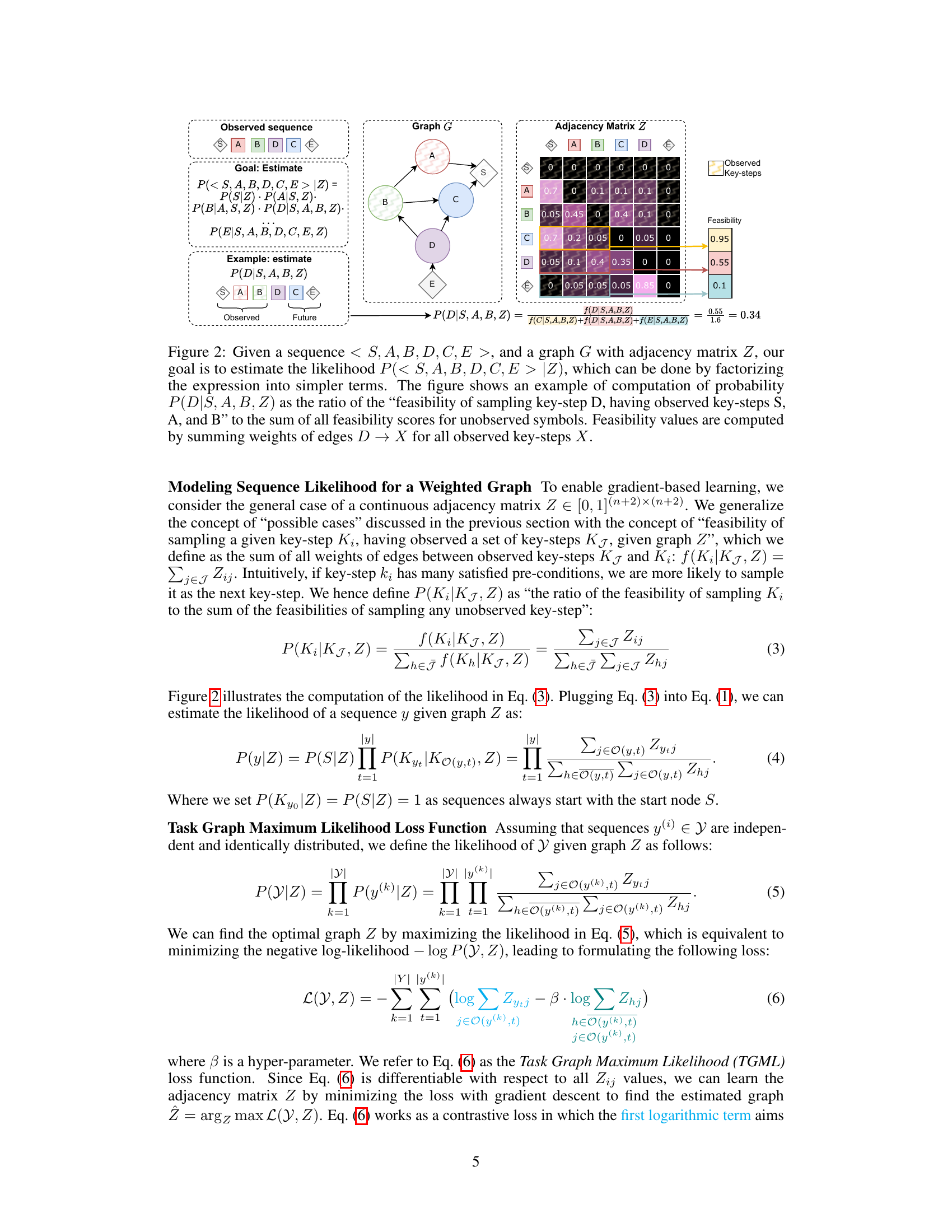
This figure illustrates how the likelihood of observing a sequence of key-steps given a task graph is computed. The likelihood is factorized into the probability of observing each key-step given the previously observed key-steps and the constraints imposed by the graph. For a weighted graph, the feasibility of sampling a given key-step is calculated as the sum of the weights of the edges from the previously observed key-steps to the given key-step. The probability of observing a key-step is then calculated as the ratio of its feasibility to the sum of the feasibilities of all unobserved key-steps.

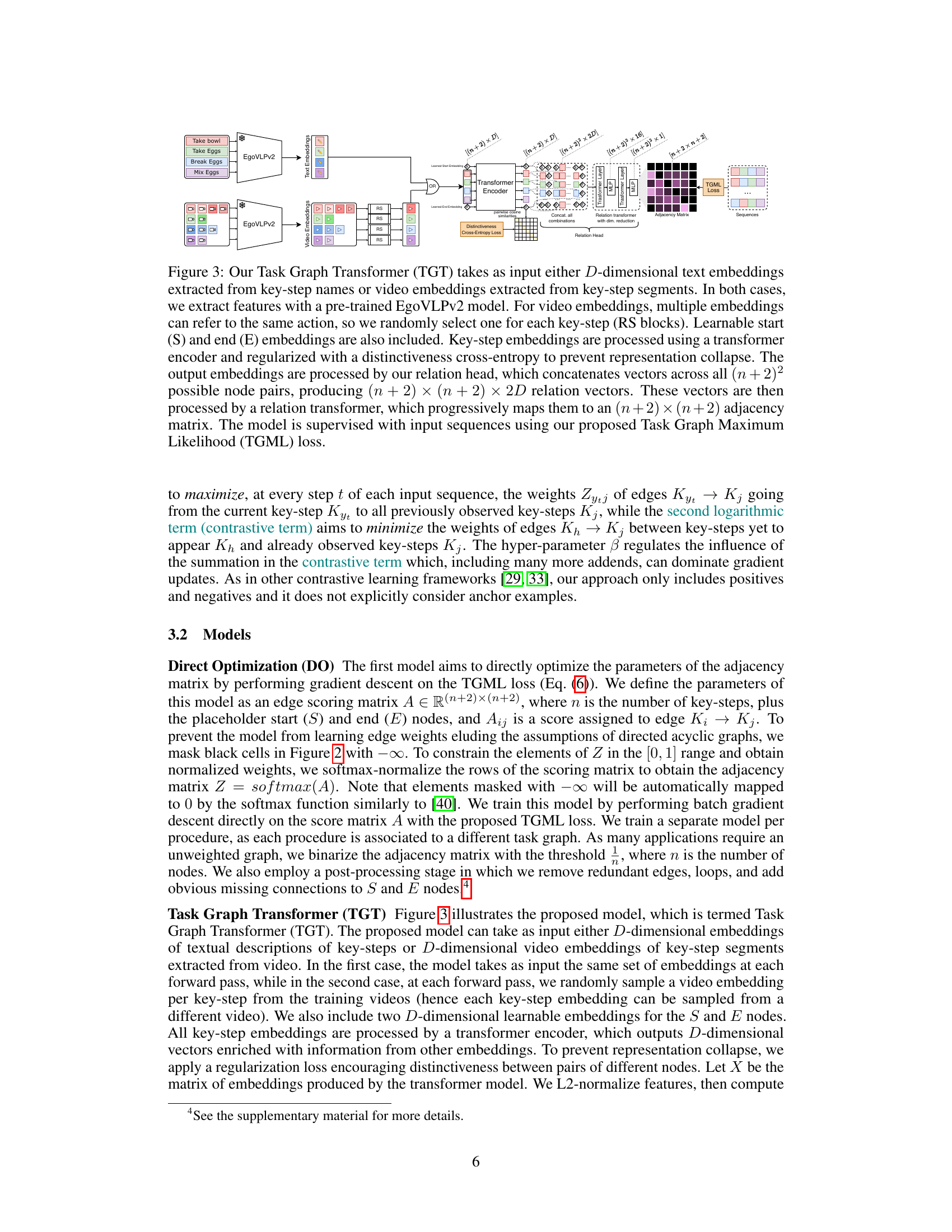
This figure illustrates the architecture of the Task Graph Transformer (TGT) model. The model takes either text or video embeddings as input, processes them using a transformer encoder, and then uses a relation head and relation transformer to predict the adjacency matrix of a task graph. A distinctiveness loss prevents overfitting, and the TGML loss ensures the predicted graph accurately reflects the input sequences.

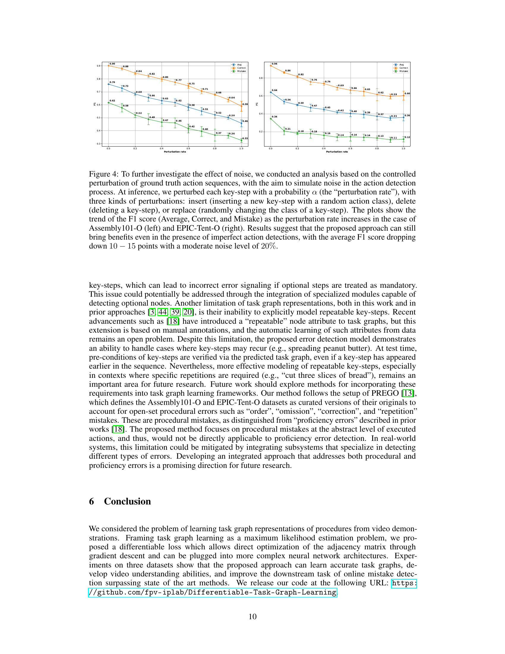
This figure shows the results of an experiment designed to test the robustness of the proposed online mistake detection method to noisy action sequences. The authors simulated noise by randomly inserting, deleting, or replacing key-steps in ground truth sequences at varying rates (perturbation rate). The resulting F1 scores (for average performance, correct predictions, and mistake predictions) are plotted against the perturbation rate for two datasets (Assembly101-O and EPIC-Tent-O). The results demonstrate that the method remains relatively effective even with a moderate level of noise.
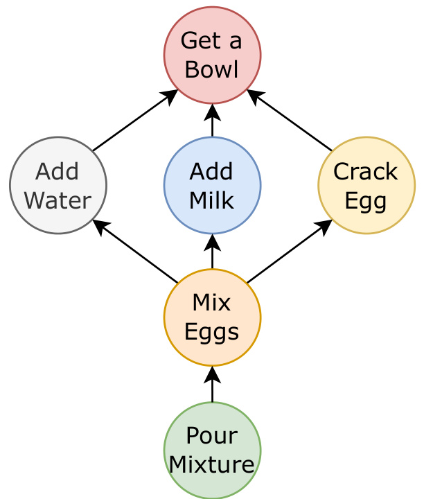
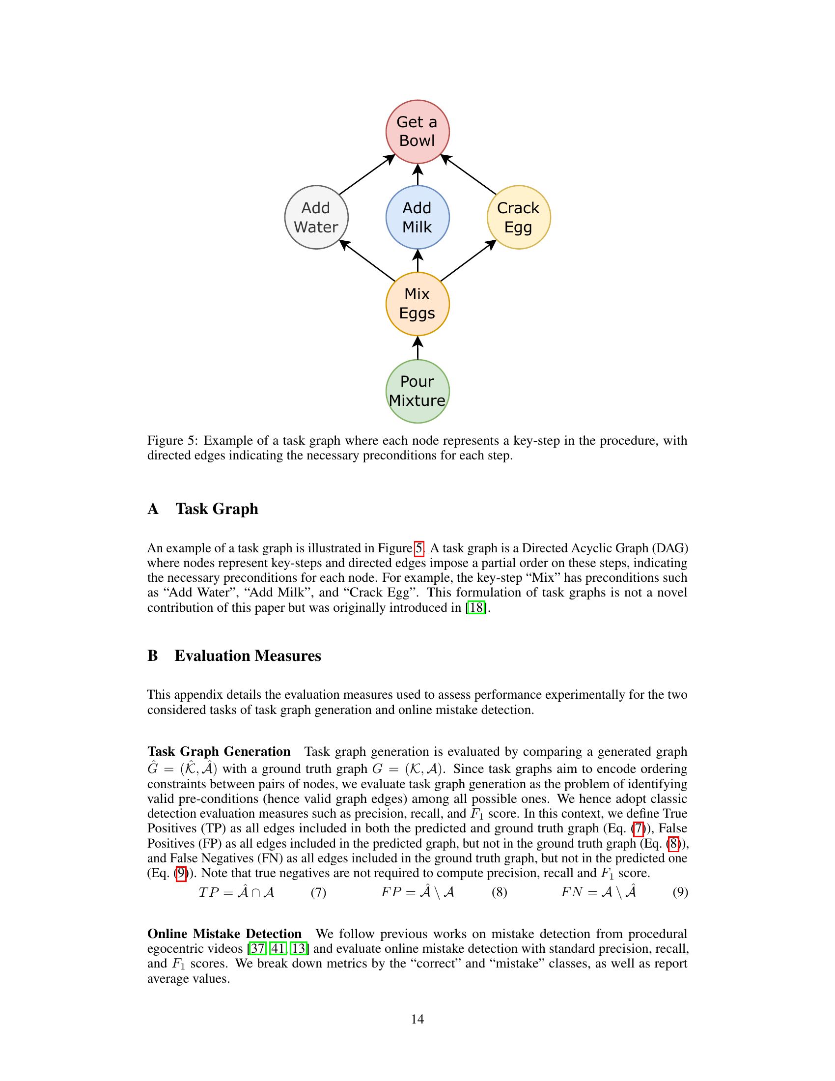
This figure shows a simple task graph representing the steps involved in a procedural task, such as making a dish. Each node (circle) represents a single step in the process, like ‘Get a Bowl’, ‘Add Water’, etc. The directed edges (arrows) show the dependencies between the steps, illustrating the order in which they must be performed. For example, ‘Mix Eggs’ requires that you have already ‘Add Water’, ‘Add Milk’, and ‘Crack Egg’. This visual representation makes it easy to understand the structure and prerequisites of a procedural activity.
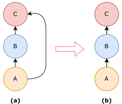
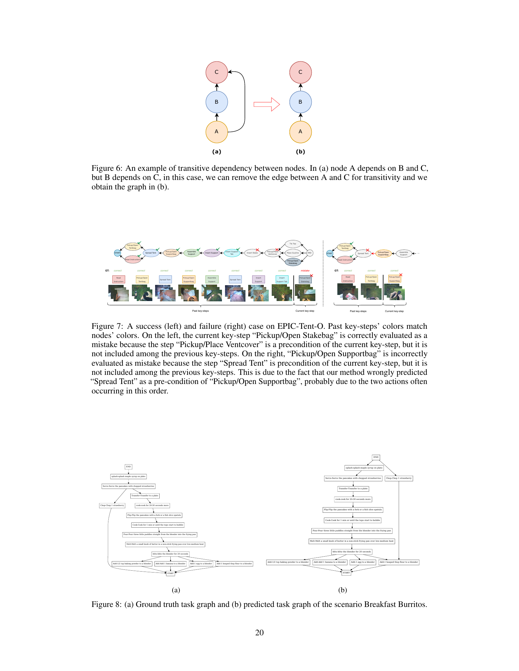
This figure shows an example of how transitive dependencies in a graph can be simplified. In the original graph (a), node A depends on both nodes B and C, and node B depends on node C. Since B’s dependency on C implies that C must also be a precondition for A, the dependency between A and C is redundant. The simplified graph (b) removes this redundant edge, resulting in a more efficient representation of the relationships between nodes.

This figure shows the effect of noise on the performance of the proposed online mistake detection method. The noise was simulated by introducing controlled perturbations (insertion, deletion, and replacement) to the ground truth action sequences at different rates. The plots show that the average F1 score decreases as the perturbation rate increases, indicating that the method is robust to noise but its performance degrades with significant noise level.
This figure illustrates how the likelihood of a sequence given a graph is computed. The likelihood is factorized into simpler probabilities for each step, considering the feasibility of sampling a key-step given previously observed steps and the graph’s constraints. The example focuses on calculating P(D|S, A, B, Z), showing the ratio of favorable cases (where D’s preconditions are met) to possible cases.

This figure illustrates how to compute likelihood of a sequence given a weighted graph by factorizing the expression into simpler terms. It gives an example of how probability of observing a key-step is estimated based on the feasibility of sampling that key-step given observed key-steps and the constraints of the graph. The feasibility is defined as the sum of all weights of edges between observed and current key-steps. The figure also shows how these probabilities are combined to estimate the likelihood of the whole sequence given the graph.

This figure illustrates how the likelihood of a sequence given a task graph is calculated. It shows how the probability of observing a specific key-step at a given position in the sequence can be factorized into simpler terms based on previously observed key-steps and the constraints encoded in the task graph. The example illustrates the calculation of P(D|S, A, B, Z), the probability of observing key-step D given that S, A, and B have already been observed.

This figure illustrates the process of calculating the probability of a sequence given a graph. It breaks down the calculation into simpler terms using factorization. The example shows how the probability of observing key-step D, given that S, A, and B have already been observed, is calculated as a ratio of its feasibility score to the sum of feasibility scores for all unobserved key-steps. This exemplifies the core idea behind the Task Graph Maximum Likelihood (TGML) loss function introduced in the paper.

This figure illustrates the concept of transitivity in directed acyclic graphs (DAGs) which are used to represent task graphs in the paper. In the left panel (a), there is a redundancy where node A depends on both B and C, but B depends on C. The right panel (b) shows the simplified, equivalent DAG resulting from removing the redundant edge A-C, thus maintaining the correct precedence relationships.

This figure illustrates how the likelihood of a sequence given a graph can be calculated by factorizing the probability into simpler terms. It gives an example that shows how to compute the probability of observing a key-step given previously observed key-steps and the constraints encoded in the graph. The feasibility of sampling a key-step is defined as the sum of all weights of edges between observed key-steps and the current key-step. This feasibility value is used to estimate the probability of the key-step appearing given the observed preconditions, which are represented in the graph.

This figure shows an example of how transitive dependencies are handled in the task graph. In the left graph (a), node A depends on both B and C, while node B depends on C. This is redundant because if B is a precondition for A and C is a precondition for B, then C is implicitly a precondition for A. The right graph (b) shows the simplified graph after removing the redundant dependency, making the graph more efficient and easier to understand.

This figure illustrates how the likelihood of a sequence of key-steps given a task graph is calculated. It uses a factorization approach, breaking down the likelihood into simpler terms representing the probability of observing each key-step given the preceding ones and the constraints encoded in the graph’s adjacency matrix. An example calculation of P(D|S, A, B, Z) is shown, highlighting the concept of ‘feasibility’ – the probability of sampling a key-step given its pre-conditions have been met.

This figure illustrates the core concept of the paper: learning task graphs from sequences of actions. (a) shows a sample task graph representing the dependencies between actions in a simple ‘mix eggs’ procedure. (b) details the proposed learning method, Task Graph Maximum Likelihood (TGML), which directly optimizes the weights of the task graph’s adjacency matrix (Z) using a contrastive loss function. This loss encourages the model to learn accurate dependencies by emphasizing the likelihood of edges connecting preceding actions to subsequent ones while suppressing the likelihood of edges from past to future actions.

The figure illustrates the architecture of the Task Graph Transformer (TGT) model. This model takes as input either text or video embeddings of key steps, processes them using a transformer encoder and a relation head, and outputs an adjacency matrix representing the task graph. The TGML loss is used to supervise the learning process.

This figure illustrates how to estimate the likelihood of a sequence given a task graph represented as an adjacency matrix. It breaks down the calculation into simpler terms by considering the probability of observing each key-step given the previously observed key-steps and the constraints encoded in the graph. It uses the concept of ‘feasibility’ to quantify the likelihood of observing a specific key-step given its preconditions. The example shows how to compute the probability P(D|S, A, B, Z), representing the probability of observing key-step D after observing S, A, and B.
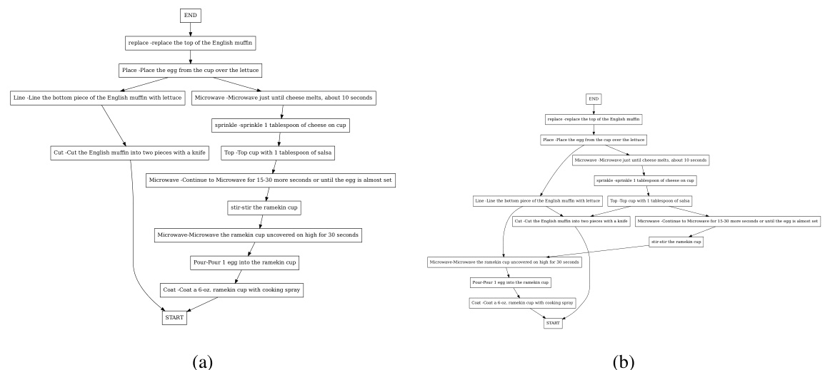
This figure shows an example of how transitive dependencies are handled in the task graph construction. In graph (a), node A depends on both B and C, while B depends on C. Because the dependency of A on C is implied through the dependency of A on B and B on C (transitivity), the edge between A and C is redundant and can be removed, resulting in the simplified graph (b). This simplification maintains the accuracy of the task graph while reducing complexity.

This figure shows a simple example of a task graph. A task graph is a directed acyclic graph (DAG) where each node represents a step in a procedure, and directed edges show the dependencies between steps. In other words, an edge from node A to node B indicates that step A must be completed before step B can begin. This particular example illustrates a common workflow for making scrambled eggs.

This figure illustrates how the likelihood of a sequence of key-steps given a graph is calculated. It shows how the probability of observing a key-step at a given position in a sequence depends on the previously observed key-steps and the constraints encoded in the graph’s adjacency matrix. The figure breaks down the computation of the conditional probability P(y|Z) into simpler terms by showing an example of calculating the probability P(D|S, A, B, Z), which is interpreted as the ratio of the ‘feasibility of sampling key-step D having observed S, A, and B’ to the sum of all feasibility scores for unobserved symbols.

This figure shows an example of how transitive dependencies can be simplified in a task graph. In the first graph (a), node A depends on both B and C, while B depends on C. Since B’s fulfillment automatically implies C’s fulfillment for A, the connection between A and C is redundant. The second graph (b) shows the simplified graph after removing this redundant edge. This simplification ensures the resulting graph maintains a directed acyclic graph (DAG) structure, crucial for representing procedural activities in the proposed framework.
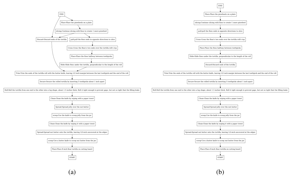
This figure illustrates the calculation of likelihood for a given sequence in a weighted graph. The likelihood is factorized into simpler terms, and the probability of observing a key-step is estimated based on the feasibility of sampling that key-step given the observed key-steps and the graph structure. The feasibility score is computed by summing weights of edges from the key-step to all observed key-steps. The example shows how to compute the probability of observing key-step D given that S, A, and B have already been observed.

This figure illustrates how to calculate the likelihood of a sequence given a graph, showing the factorization of the probability into simpler terms. It also demonstrates how the probability of a specific key-step (D) is computed given previously observed key-steps (S, A, B) and the constraints encoded in the graph’s adjacency matrix (Z). The ‘feasibility’ calculation represents the sum of edge weights from observed nodes to the current node under consideration.

This figure illustrates the architecture of the Task Graph Transformer (TGT) model, which takes either text or video embeddings as input and predicts a task graph represented as an adjacency matrix. It uses a transformer encoder, a relation head, and a relation transformer to process the embeddings and predict the adjacency matrix. The model is trained with the proposed TGML loss function.

This figure demonstrates a graph simplification process that handles transitive dependencies. The original graph (a) shows node A depending on both nodes B and C, while node B in turn depends on node C. Because B’s existence implies C’s, the direct dependency between A and C is redundant. The simplified graph (b) removes this unnecessary edge, resulting in a more efficient and accurate representation of the relationships.

This figure shows an example of how transitive dependencies can be simplified in a directed acyclic graph (DAG). The figure depicts two graphs: (a) shows a scenario where node A depends on both nodes B and C, and node B depends on node C; (b) shows the simplified graph after removing the redundant edge between A and C because the dependency is already implied by the path A -> B -> C. This simplification is done to ensure that the resulting graph remains a DAG.

This figure illustrates how the likelihood of a sequence given a graph is computed. It breaks down the calculation into smaller, more manageable parts and shows how the probability of each step is influenced by the previous steps and the structure of the graph. The figure highlights the concept of ‘feasibility’ in determining the probability of observing a specific key-step at a given point in the sequence. It showcases a practical example to clarify the process.
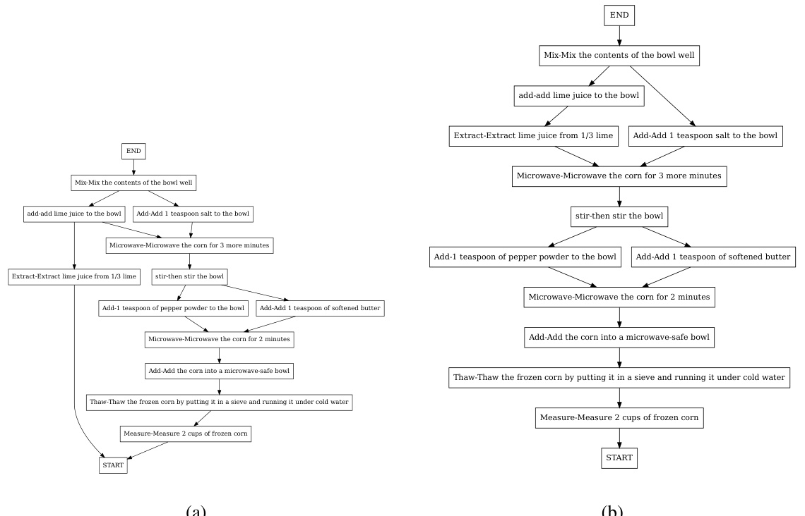
This figure shows an example of how to simplify a task graph by removing redundant edges. In the first graph (a), node A depends on both nodes B and C, and node B depends on node C. Because of the transitive nature of dependencies, the link between A and C is unnecessary. The simplified graph (b) removes this redundancy.

This figure shows an example of how transitive dependencies between nodes in a graph can be simplified. In the first graph (a), node A depends on both nodes B and C, while node B depends on node C. Since the dependency is transitive (B is a precondition for A, and C is a precondition for B, therefore C is also a precondition for A), the edge between A and C is redundant. Removing this redundant edge simplifies the graph to graph (b). This process of removing redundant edges helps to ensure that the graph is a directed acyclic graph (DAG), representing the partial ordering of tasks in a clear and concise manner.

This figure shows an example of how transitive dependencies are handled in the task graph. The graph in (a) shows node A depending on nodes B and C, while node B depends on node C. Since the dependency of A on C is implied through the dependency of A on B and B on C, the edge between A and C is redundant and can be removed to simplify the graph, resulting in the graph shown in (b). This process ensures that the task graph remains a directed acyclic graph (DAG), maintaining the correctness of the partial ordering of key-steps.
More on tables
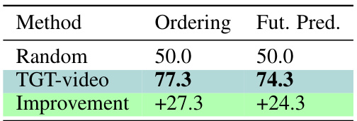
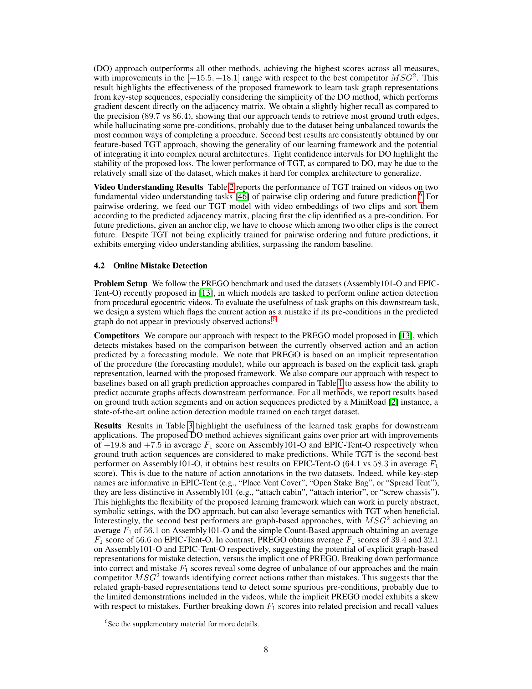
This table compares the performance of the TGT model (trained on visual features) on two video understanding tasks: pairwise ordering and future prediction. It shows the model’s accuracy on these tasks, along with the improvement over a random baseline. The results demonstrate that the model, despite not being explicitly trained for these tasks, exhibits video understanding abilities, surpassing the baseline.
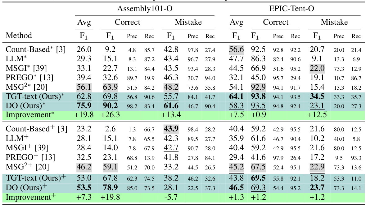
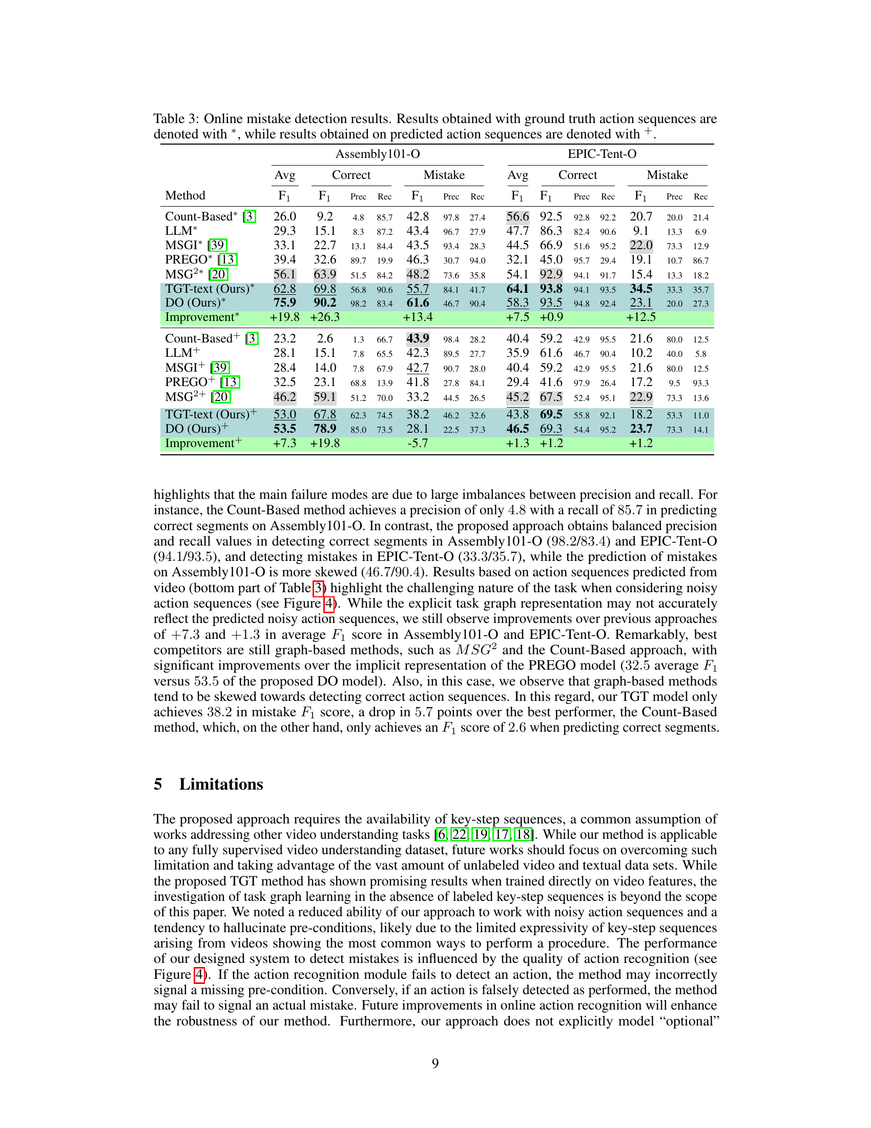
This table presents the performance of different methods on the online mistake detection task using two datasets (Assembly101-O and EPIC-Tent-O). The results are broken down into average F1 scores, and further subdivided by correct and mistake predictions, reporting precision and recall for each. Results are shown for both scenarios where ground truth action sequences are used and where predicted action sequences are used. The ‘Improvement’ row shows the improvement in average F1 score over the PREGO baseline method. The table highlights the effectiveness of the proposed method, DO, in comparison to the other approaches in terms of accuracy and robustness in the online mistake detection task.
This table presents the performance of different methods for task graph generation on the CaptainCook4D dataset. The metrics used are precision, recall, and F1-score, which are common metrics for evaluating the accuracy of classification tasks. The table highlights the best performing method among all the compared approaches and indicates the confidence intervals for the results, which helps to assess the reliability of the performance measurements.

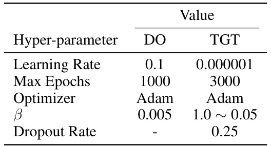
This table lists the hyperparameters used for training the Direct Optimization (DO) and Task Graph Transformer (TGT) models on the Assembly101-O and EPIC-Tent-O datasets. It shows the learning rate, maximum number of training epochs, optimizer used (Adam), beta (β) parameter for the TGML loss, and dropout rate (only applicable to the TGT model). Note that the beta parameter is linearly annealed from 1.0 to 0.55 during training for the TGT model.

This table presents the performance comparison of different methods for task graph generation on the CaptainCook4D dataset. The metrics used for evaluation are precision, recall, and F1-score. The table highlights the best performing method, indicating the improvements achieved over existing approaches. Confidence intervals are also provided to demonstrate the reliability and statistical significance of the results.

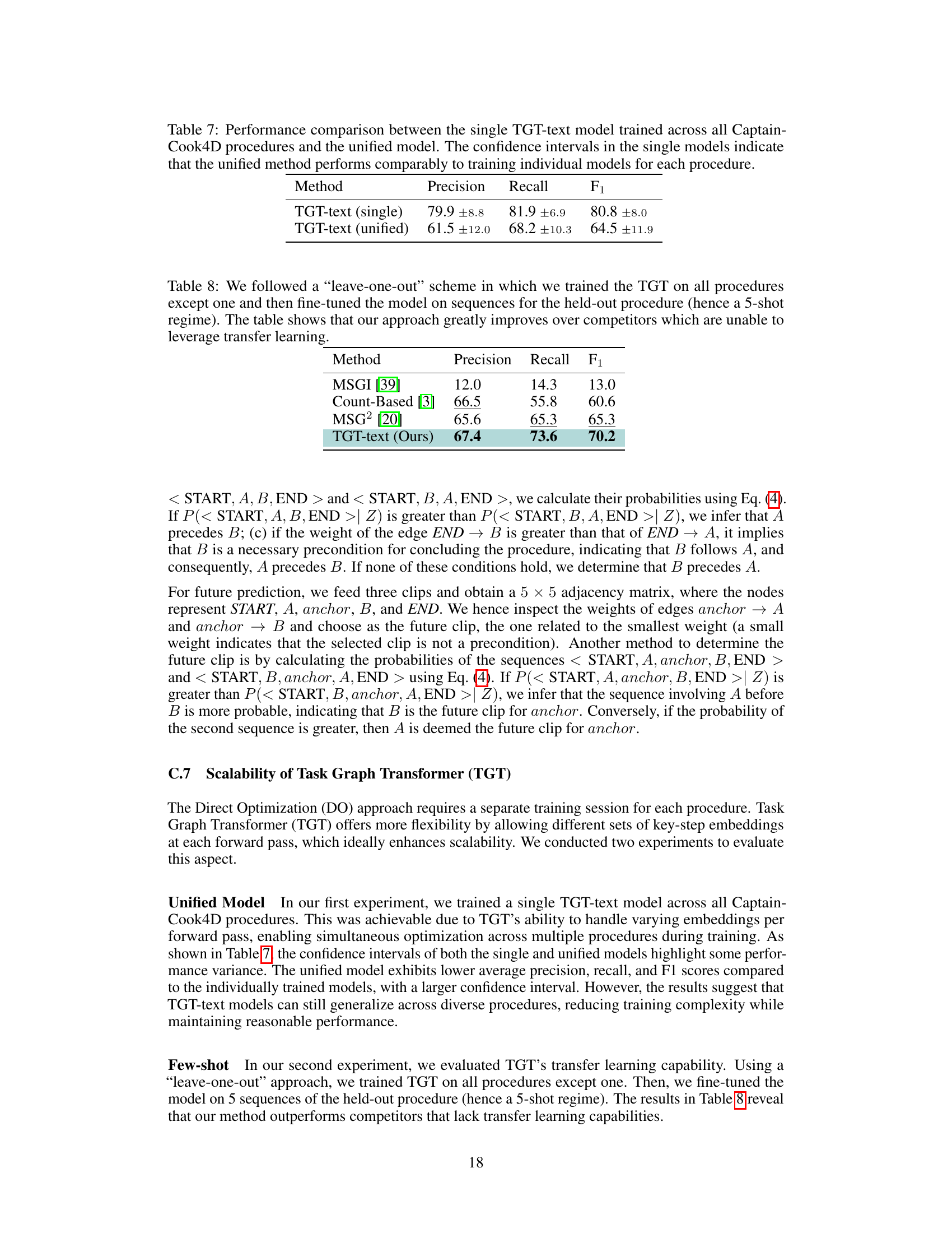
This table compares the performance of two different approaches for training a Task Graph Transformer (TGT) model for task graph generation on the CaptainCook4D dataset. The first approach trained a separate TGT model for each of the 24 procedures in the dataset. The second approach trained a single unified TGT model across all 24 procedures. The table shows that while the unified model shows slightly lower precision, recall, and F1 scores than the average of the individual models, the confidence intervals indicate that the performance difference is not statistically significant.

This table compares the performance of the proposed TGT model with other state-of-the-art methods on the task of task graph generation using a leave-one-out cross-validation approach. It demonstrates the effectiveness of the transfer learning capability of the TGT model by showing significant improvement in performance compared to methods that don’t utilize transfer learning.
Full paper#

