↗ OpenReview ↗ NeurIPS Proc. ↗ Chat
TL;DR#
Many machine learning applications deal with data from multiple sources, each providing small batches of samples insufficient for individual model training. A common approach assumes these sources belong to several subgroups, each with its own characteristics. This approach is problematic when dealing with long-tailed distributions common in applications like federated learning and recommendation systems, as many sources provide very little data. Prior work requires strict assumptions like isotropic Gaussian distributions for all subgroups, limiting practical applicability. The problem is further complicated by limited labeled samples in most batches.
This paper introduces a novel gradient-based algorithm that overcomes these limitations. The algorithm allows for different, unknown, and heavy-tailed input distributions across subgroups, and it recovers subgroups even with a large number of sources. It improves sample and batch size requirements and relaxes the need for separation between regression vectors. The algorithm’s effectiveness is validated through theoretical guarantees and empirical results showing significant improvements over previous methods, highlighting its potential to improve personalization and accuracy in various applications.
Key Takeaways#
Why does it matter?#
This paper is crucial for researchers working with heterogeneous data batches, particularly in federated learning, sensor networks, and recommendation systems. It offers significant improvements in accuracy and efficiency compared to existing methods, opening new avenues for personalized models even with limited data per source. Addressing the challenges of non-isotropic and heavy-tailed input distributions, this work broadens the applicability of linear regression techniques and encourages exploration of alternative gradient-based algorithms.
Visual Insights#
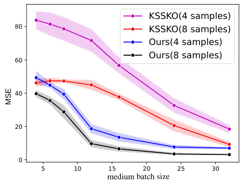
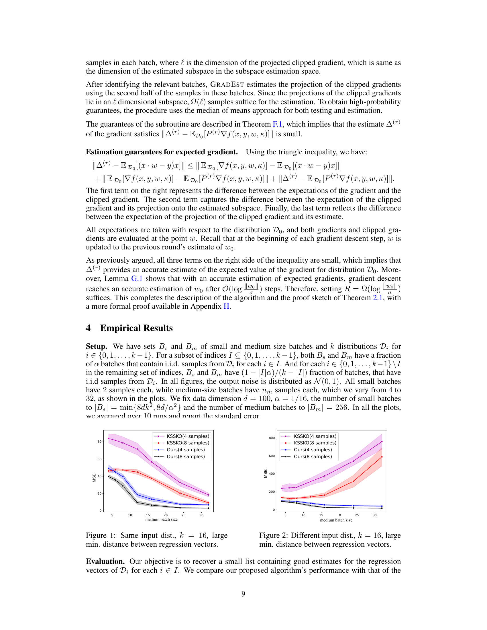
The figure compares the performance of the proposed algorithm with that of the algorithm in [KSS+20] under the same setting as in [KSS+20], i.e., with more restrictive assumptions. The results show that the proposed algorithm significantly outperforms [KSS+20] in terms of MSE, especially for smaller medium batch sizes.
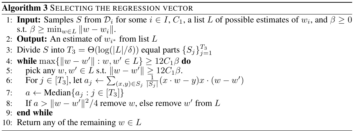
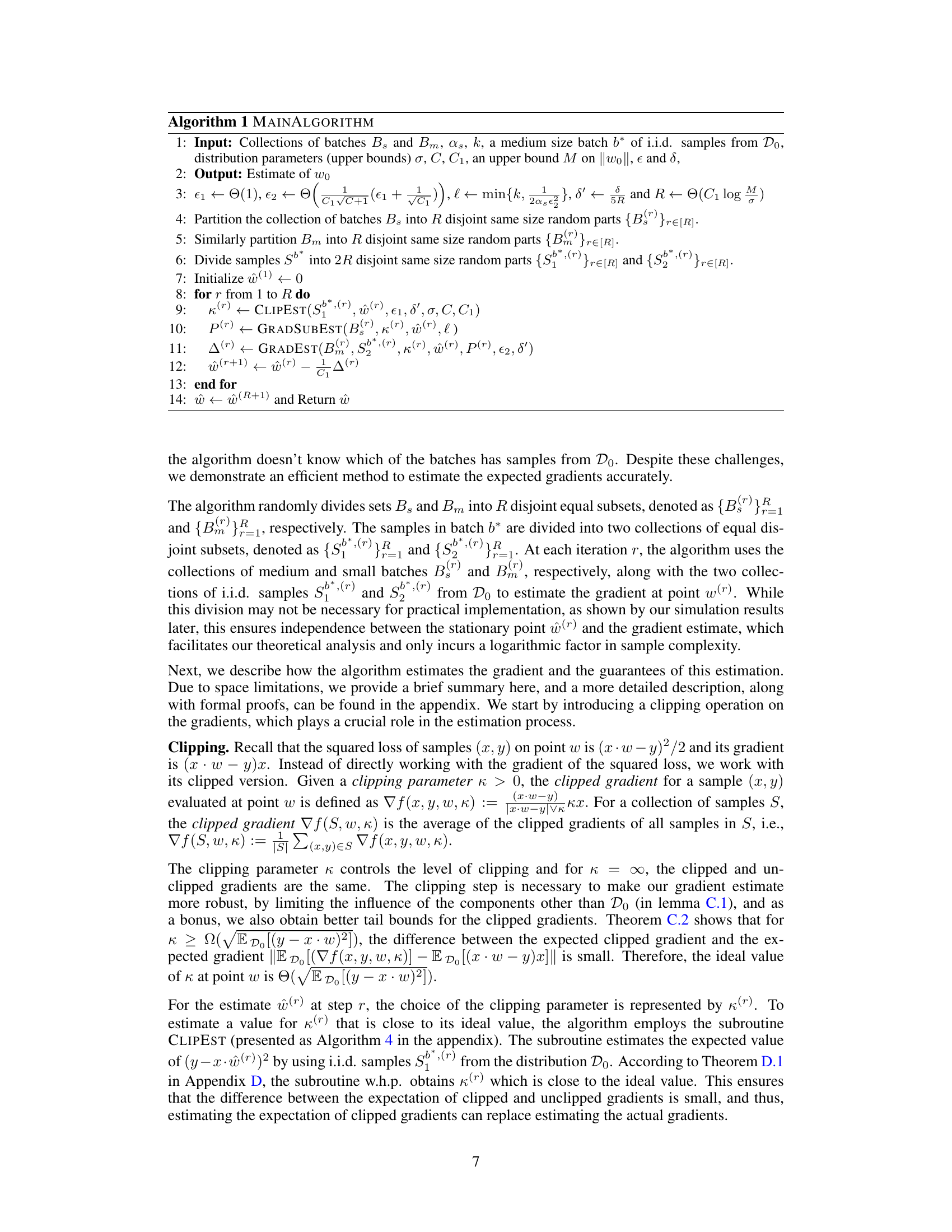
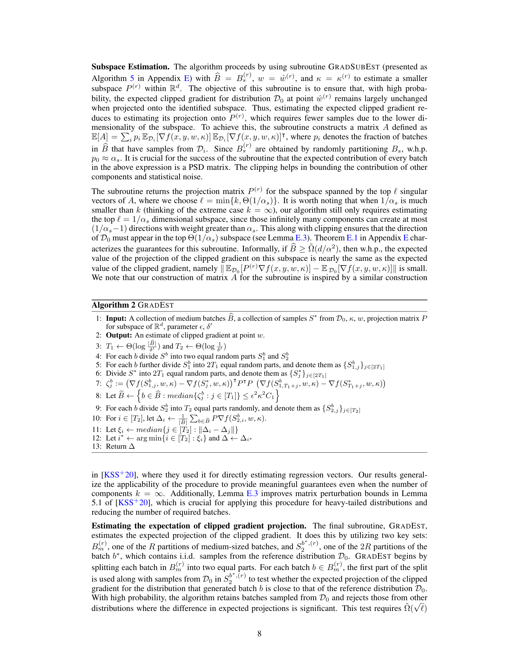
This algorithm selects the regression vector from a given list L that is closest to the true regression vector w*. It iteratively removes elements from L until all the remaining elements are close to each other. The algorithm uses samples from Di and the list L to estimate a smaller subspace that preserves the norm of the gradient for sub-population i, reducing the minimum length of medium-size batches required for testing and the number of medium-size batches required for estimation. The algorithm runs in polynomial-time and has a sample complexity that is within a factor of Õ(1/a) from that required in a single-component setting.
In-depth insights#
Heterogeneous Batch#
The concept of “Heterogeneous Batch” in machine learning signifies handling data batches exhibiting variability in their underlying data distributions. This contrasts with the traditional assumption of homogeneity, where each batch is drawn from an identical distribution. This heterogeneity arises naturally in many real-world applications where data are collected from diverse sources and under different conditions. A key challenge is that standard learning algorithms often fail when presented with such diverse data. Addressing heterogeneous batches necessitates techniques that can either identify and separate the underlying distributions or develop robust learning methods capable of adapting to various distributional characteristics. Strategies include clustering similar batches together and training separate models, developing robust loss functions less sensitive to outliers, or employing meta-learning approaches to learn across different distributions. Efficient and accurate methods for handling heterogeneous batches are essential for improving the generalization capabilities and performance of machine learning models in complex real-world scenarios. The choice of approach depends critically on the nature of the heterogeneity and the computational resources available.
Gradient-Based Algo#
A gradient-based algorithm offers a powerful approach to solving optimization problems, particularly in machine learning. Its core strength lies in its iterative nature; it refines its solution gradually by following the negative gradient of the objective function. This method is especially valuable when dealing with complex, non-convex functions, where traditional methods may struggle. The algorithm’s effectiveness depends heavily on several factors, including the choice of learning rate (step size), which determines the magnitude of each update, and the initialization of the algorithm’s parameters. A poorly chosen learning rate can lead to slow convergence or divergence. Careful consideration must also be given to the optimization landscape. Local minima and saddle points can hinder the algorithm’s progress, necessitating techniques like momentum or adaptive learning rates to escape such regions. Furthermore, the algorithm’s computational complexity is an important consideration. Each iteration involves computing the gradient, which can be expensive for high-dimensional problems. Therefore, efficient gradient computation methods are often crucial for practical applications. Lastly, the choice of objective function itself plays a significant role. A poorly designed objective function can yield suboptimal results. In summary, a well-designed and carefully tuned gradient-based algorithm can be extremely effective, but requires attention to detail regarding numerous aspects of its design and implementation.
Heavy-tailed Data#
The concept of heavy-tailed data is crucial in robust statistical modeling because it acknowledges that real-world datasets often deviate significantly from the idealized assumption of normality. Many machine learning algorithms implicitly assume Gaussian distributions, which can lead to inaccurate results when applied to datasets with heavy tails. Heavy-tailed distributions, characterized by extreme values occurring more frequently than predicted by a Gaussian model, pose unique challenges to conventional statistical methods. Outliers, a common feature of heavy-tailed data, can disproportionately affect the results of standard estimation techniques like least squares regression. Addressing heavy-tailed data requires robust methods that are less sensitive to extreme values, including approaches like median-based estimators, M-estimators, or robust regression techniques. Understanding the nature of heavy tails (e.g., the specific distribution, the prevalence of extreme values) is critical for selecting the appropriate model and ensuring reliable results. Furthermore, careful data preprocessing techniques, such as outlier detection and winsorization, can mitigate the negative impact of outliers on the analysis. The presence of heavy-tailed data highlights the necessity of employing robust and resistant statistical methods in data analysis.
Prior Work Contrast#
The ‘Prior Work Contrast’ section of a research paper is crucial for establishing the novelty and significance of the presented work. A strong contrast highlights key improvements over existing methods, showcasing not just incremental advancements but substantial leaps forward. This involves a detailed comparison of assumptions, algorithms, and results, emphasizing where the new approach excels. It’s important to go beyond superficial comparisons. A truly effective contrast focuses on fundamental differences, explaining why previous methods might fail in certain scenarios where the new one succeeds. This could involve discussions on computational complexity, sample size requirements, robustness to noise or outliers, or the ability to handle high dimensionality or complex data distributions. Highlighting limitations of previous works is important but should be balanced with a clear demonstration of how the new approach overcomes those limitations. A thoughtful analysis of related works helps position the research within the broader landscape, building a convincing case for its contribution to the field. Finally, it should clearly articulate the unique aspects of the new approach that differentiate it from what came before, making a clear case for its novelty and potential impact.
Future Directions#
Future research could explore several promising avenues. Extending the algorithm to handle non-linear relationships would significantly broaden its applicability, potentially using kernel methods or neural networks to adapt to more complex data structures. Investigating the algorithm’s robustness to different noise models beyond additive Gaussian noise is crucial. Addressing scenarios with missing data or imbalanced classes would also enhance its practicality. Furthermore, a deeper theoretical analysis to refine the sample complexity bounds and runtime could lead to more efficient algorithms. Developing more efficient gradient estimation techniques and exploring alternative optimization methods might improve performance, particularly for high-dimensional data. Finally, applying the algorithm to a wider range of real-world applications, such as personalized recommendation systems or federated learning, is essential to validate its effectiveness and practical utility. The evaluation metrics should also be rigorously extended to better capture the complexities of real-world applications.
More visual insights#
More on figures
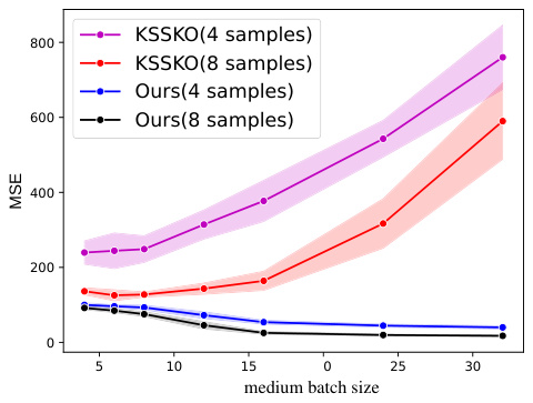
The figure shows the mean squared error (MSE) for different medium batch sizes when comparing the proposed algorithm with the KSS+20 algorithm. The input distributions are the same for all sub-populations, the number of sub-populations is 16, and there is a large minimum distance between the regression vectors. The plot shows the MSE for new batches of size 4 and 8, averaged over 10 runs. The error bars represent standard errors.
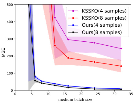
This figure compares the performance of the proposed algorithm and the KSSKO algorithm on a linear regression task with 16 sub-populations. The input distributions are identical across all sub-populations, and the regression vectors are well-separated (large minimum distance). The plot shows the mean squared error (MSE) achieved by each algorithm for different medium batch sizes and new batch sizes of 4 and 8. The shaded regions represent the standard error over multiple runs.
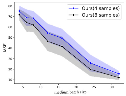
This figure compares the performance of the proposed algorithm with the algorithm from [KSS+20] under more restrictive assumptions. Specifically, it shows the Mean Squared Error (MSE) for both algorithms across different medium batch sizes (4 and 8 samples per batch). The results demonstrate that the proposed algorithm significantly outperforms the baseline, even under these restrictive conditions where all input distributions are identical, and there’s a large separation between regression vectors.
Full paper#
