↗ OpenReview ↗ NeurIPS Proc. ↗ Chat
TL;DR#
Time series analysis faces challenges in handling complex periodic variations and the limitations of existing methods. Traditional methods struggle to capture multi-level periodic relationships and often overlook the inherent hierarchical structure within time series data. This results in suboptimal performance for many real-world applications such as weather forecasting and traffic prediction, where multi-periodic patterns are common.
To overcome these limitations, this paper introduces Peri-midFormer, which decomposes a time series into a periodic pyramid. This pyramid structure explicitly represents inclusion and overlap relationships between periodic components of varying lengths. Peri-midFormer leverages self-attention within this pyramid structure to capture complex temporal dependencies between these components. Experiments show that Peri-midFormer significantly outperforms state-of-the-art methods on various time-series tasks, highlighting the efficacy of its approach.
Key Takeaways#
Why does it matter?#
This paper is crucial for researchers in time series analysis due to its novel approach to modeling multi-periodicity. Peri-midFormer’s superior performance across five mainstream tasks (forecasting, imputation, classification, and anomaly detection) and its efficiency make it a significant contribution. It opens new avenues for research in complex temporal pattern extraction and hierarchical feature representation, particularly relevant to real-world applications with intricate periodic variations.
Visual Insights#

This figure illustrates the concept of multi-periodicity in time series, where variations occur at multiple periodic levels (e.g., yearly, monthly, weekly, daily). It shows how these variations are not independent but rather exhibit inclusion relationships, with longer periods encompassing shorter ones. This is represented as a periodic pyramid structure, where the original time series is at the top level, and subsequent levels consist of periodic components with gradually shorter periods. This pyramid-like structure helps to explicitly represent the complex relationships between periodic variations within the time series.

This table presents the results of the long-term forecasting experiments on eight real-world benchmark datasets. The metrics used are Mean Squared Error (MSE) and Mean Absolute Error (MAE). The results are averaged across four different forecasting lengths (96, 192, 336, and 720 time steps). The table compares the Peri-midFormer model against several other state-of-the-art models and highlights the best and second-best performing models in red and blue, respectively.
In-depth insights#
Periodic Pyramid#
The concept of a “Periodic Pyramid” in time series analysis offers a novel approach to handle the complexity of multi-periodic data. Instead of treating a time series as a flat sequence, it structures the data hierarchically, with each level of the pyramid representing periodic components of a specific frequency. This structure elegantly captures the inclusion and overlap relationships among different periodicities, such as daily variations nested within weekly and yearly cycles. Self-attention mechanisms can then be applied across the pyramid’s levels, enabling the model to capture long-range dependencies and complex interactions among components at different scales. This hierarchical approach is beneficial because it provides a multi-resolution representation of temporal variations, allowing the model to learn both fine-grained and coarse-grained temporal patterns. Ultimately, the effectiveness hinges on the ability to accurately decompose the original time series into meaningful periodic components and effectively leverage the pyramidal structure for feature extraction.
Transformer Design#
The effective design of Transformers for time series analysis hinges on several key considerations. Addressing the inherent sequential nature of time series data is crucial, often necessitating modifications to standard Transformer architectures. This might involve incorporating specialized positional encodings that better capture temporal dependencies or employing recurrent mechanisms to enhance the model’s ability to learn long-range relationships. Another critical aspect is handling the varying lengths and complexities of time series; techniques like attention mechanisms with adjustable receptive fields or hierarchical architectures can improve model performance and efficiency. Furthermore, optimizing the model for specific time series tasks, like forecasting or classification, may require unique adaptations to the Transformer’s output layer and loss function. Finally, balancing computational efficiency and model accuracy remains a significant challenge, prompting the exploration of efficient attention mechanisms, model compression techniques, and hardware-aware design choices to minimize computational costs without sacrificing predictive performance.
Multi-task Results#
A dedicated ‘Multi-task Results’ section would offer a powerful demonstration of the model’s versatility. By showcasing performance across diverse tasks—forecasting (short and long-term), imputation, classification, and anomaly detection—the study could highlight the model’s adaptability and generalizability. Direct comparison to existing state-of-the-art methods on each task is vital, using standardized metrics for each to allow for fair evaluation. Visualizations like bar charts or radar plots would effectively summarize the performance across tasks, potentially showing the model’s strengths and weaknesses. The discussion should delve into the factors driving the model’s success or failure on different tasks, relating findings back to the core methodology of the model. This would strengthen the overall impact and provide valuable insights into practical applications of the approach. Statistical significance should be clearly indicated for the reported results. Presenting confidence intervals and addressing any potential biases related to the dataset selections would ensure robustness.
Ablation Studies#
Ablation studies systematically remove components of a model to assess their individual contributions. In the context of a time series analysis model like Peri-midFormer, this might involve removing the periodic pyramid structure, the periodic pyramid attention mechanism (PPAM), or the periodic feature flow aggregation. The results would reveal the relative importance of each component in achieving the overall performance. For instance, removing the PPAM might significantly decrease performance on tasks requiring complex temporal dependency understanding, while removing the periodic pyramid itself might show the importance of multi-periodicity modeling. A well-designed ablation study should provide quantitative and qualitative insights, demonstrating the strengths and weaknesses of each architectural choice and guiding future improvements. The ablation study’s findings could illuminate whether the model’s success stems primarily from its novel architectural components or from other factors such as data preprocessing or the choice of hyperparameters. By carefully controlling experimental conditions and comparing performance metrics across various ablation scenarios, researchers can draw robust conclusions about the impact of each model component on performance.
Future Works#
The paper’s conclusion briefly mentions future work, suggesting avenues for improvement. A crucial area is addressing limitations in scenarios where periodicity is weak or absent. The current model’s reliance on periodic components might hinder performance on datasets dominated by trends or noise. Further investigation into enhancing the model’s ability to handle non-periodic time series would significantly broaden its applicability. Exploring alternative decomposition methods, beyond FFT, could also be beneficial, potentially enabling the model to capture different types of temporal patterns more effectively. Comparative analysis of different attention mechanisms, beyond PPAM, is warranted to explore if other architectures can offer performance improvements or reduce computational costs. Finally, deeper exploration of the model’s scalability and its potential for handling high-dimensional, multi-variate time series is needed to fully assess its real-world potential.
More visual insights#
More on figures
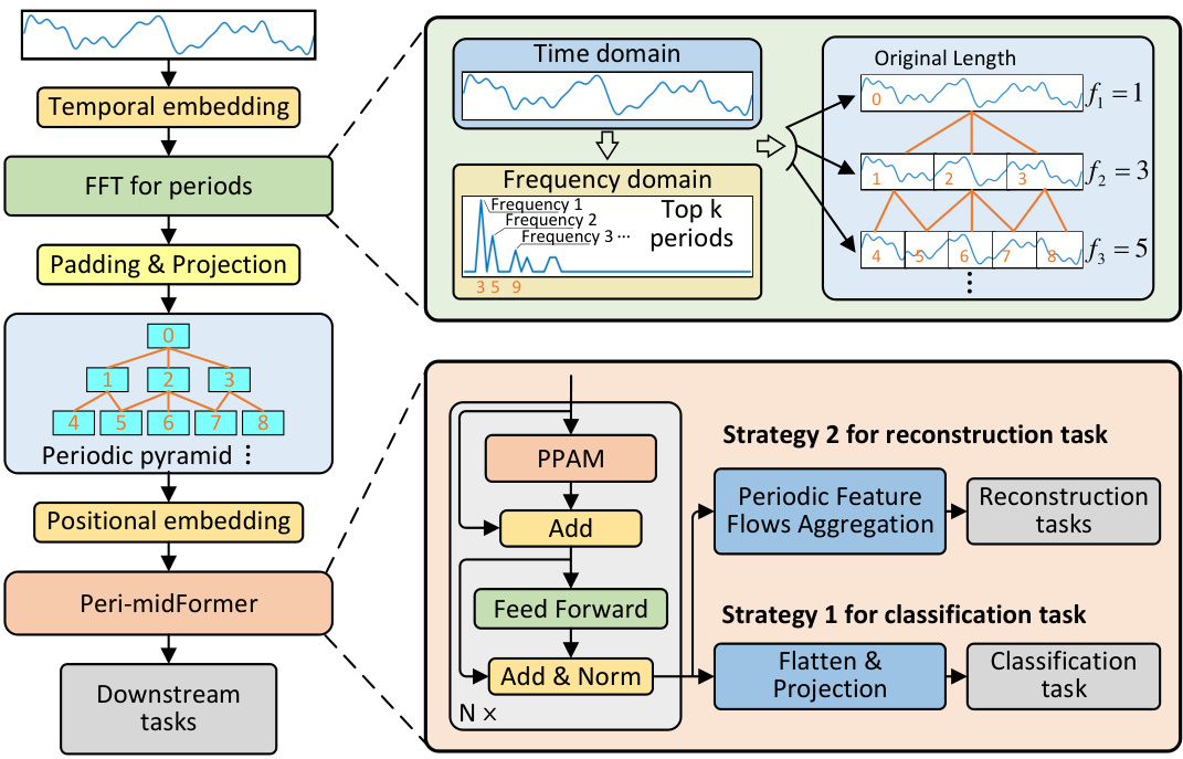
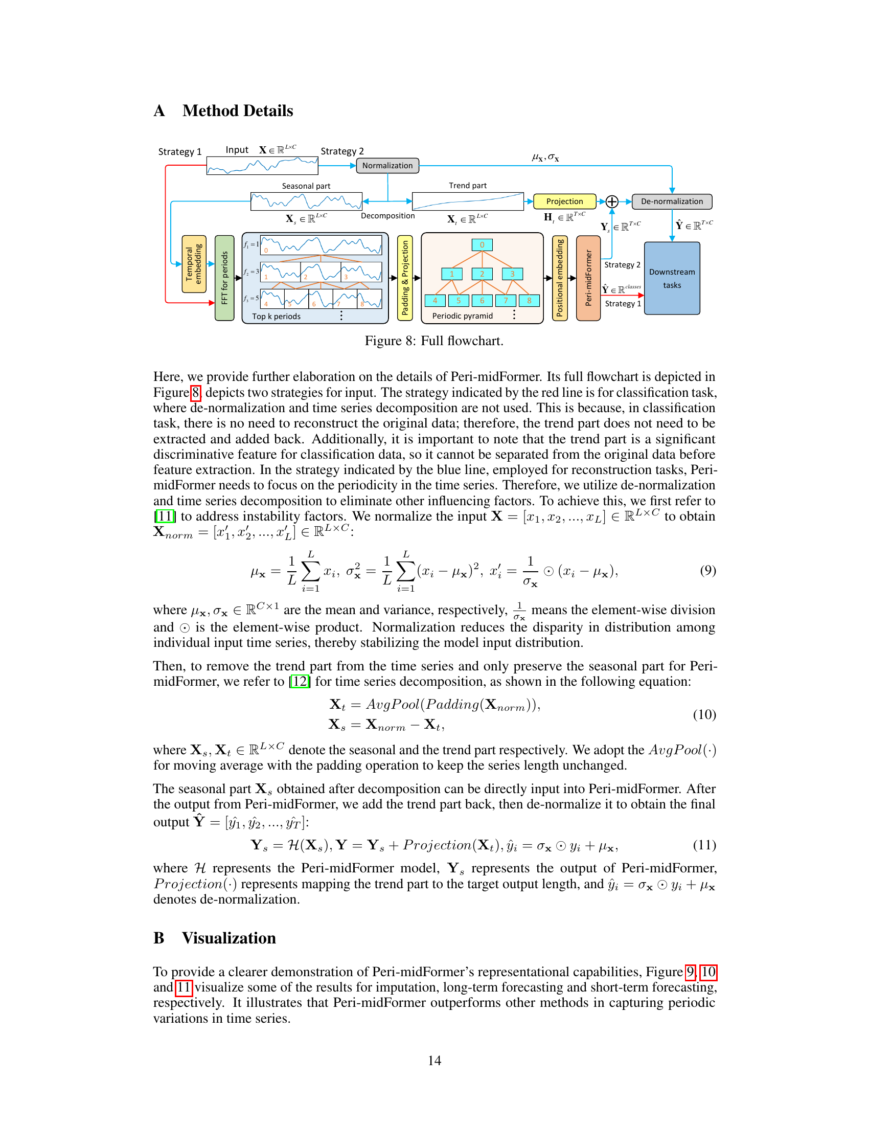
This figure illustrates the architecture of the Peri-midFormer model. The model starts by taking the original time series as input and then decomposing it using FFT into multiple periodic components of varying lengths. These components are organized into a periodic pyramid structure, with longer periods encompassing shorter ones. The periodic pyramid is then fed into a Peri-midFormer module which uses a Periodic Pyramid Attention Mechanism (PPAM) to capture complex temporal variations by computing self-attention between periodic components. Finally, depending on the downstream task (classification or reconstruction tasks), different strategies are employed to aggregate the features from the pyramid and produce the final output.

This figure illustrates the concept of multi-periodicity in time series, where multiple periodic components with different periods exist and overlap with each other. The inclusion relationships between components are shown, where longer periods contain shorter periods. The figure introduces the ‘Periodic Pyramid’ structure, where the top level represents the original time series, and lower levels represent periodic components with gradually shorter periods. This pyramid-like structure explicitly shows the implicit multi-period relationships within a time series.

This figure illustrates the overall architecture of the Peri-midFormer model. It starts with time embedding of the original time series. Then, it uses the FFT to decompose it into multiple periodic components of varying lengths across different levels, forming the Periodic Pyramid. Each component is treated as an independent token and receives positional embedding. Next, the Periodic Pyramid is fed into Peri-midFormer, consisting of multiple layers for computing Periodic Pyramid Attention. Finally, depending on the task, two strategies are employed. For classification, components are directly concatenated and projected into the category space; for reconstruction tasks, features from different pyramid branches are integrated through Periodic Feature Flows Aggregation to generate the final output.

This radar chart compares the performance of Peri-midFormer against other state-of-the-art time series analysis methods across five common tasks: long-term forecasting, short-term forecasting, imputation, classification, and anomaly detection. Each axis represents a task, and the distance from the center to a point on a line indicates the performance (lower MSE for forecasting and imputation, higher accuracy for classification, and higher F1-score for anomaly detection) on that specific task. Peri-midFormer demonstrates superior performance across all five tasks, consistently outperforming other methods.

This figure shows a bar chart comparing the average classification accuracy of Peri-midFormer and various baseline models across 10 subsets of the UEA benchmark dataset. The chart visually represents the superior performance of Peri-midFormer compared to other methods, highlighting its effectiveness in time series classification tasks.

This figure compares the performance of Peri-midFormer against other state-of-the-art time series analysis models across five benchmark tasks: long-term forecasting, short-term forecasting, classification, imputation, and anomaly detection. Each task’s performance is represented on a separate axis of a radar chart, enabling a visual comparison of the models’ overall capabilities. Peri-midFormer demonstrates superior performance in most cases, indicating its robustness and effectiveness across different tasks. The models’ names are given as labels on the radar chart, and specific metrics (e.g., MSE, accuracy, F1-score) are specified for each axis to represent quantitative performance measurements.
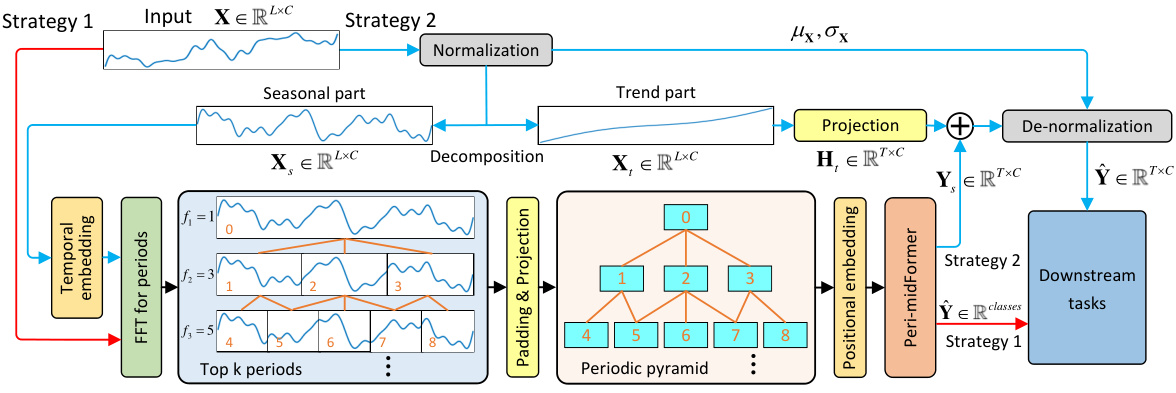
This figure illustrates the architecture of the Peri-midFormer model. It shows the input time series undergoing normalization and decomposition into trend and seasonal components. The seasonal component is then processed using FFT to extract multiple periodic components at different levels, creating a Periodic Pyramid structure. These components are passed into the Peri-midFormer which uses a Periodic Pyramid Attention Mechanism (PPAM) to capture relationships between components at different levels. Finally, the processed features are used for downstream tasks using one of two strategies: direct concatenation and projection for classification tasks; or reconstruction tasks which incorporate features from multiple flows via a Periodic Feature Flows Aggregation.

This figure shows the overall architecture of the proposed Peri-midFormer model. It starts with the time embedding of the original time series, followed by a Fast Fourier Transform (FFT) to decompose the series into multiple periodic components. These components are then organized into a Periodic Pyramid structure, which is further processed by the Periodic Pyramid Attention Mechanism (PPAM). Finally, depending on the downstream task (classification or reconstruction), different strategies are used to generate the final output. The figure clearly illustrates the inclusion relationships between different levels of periodic components and the overall flow of information through the model.

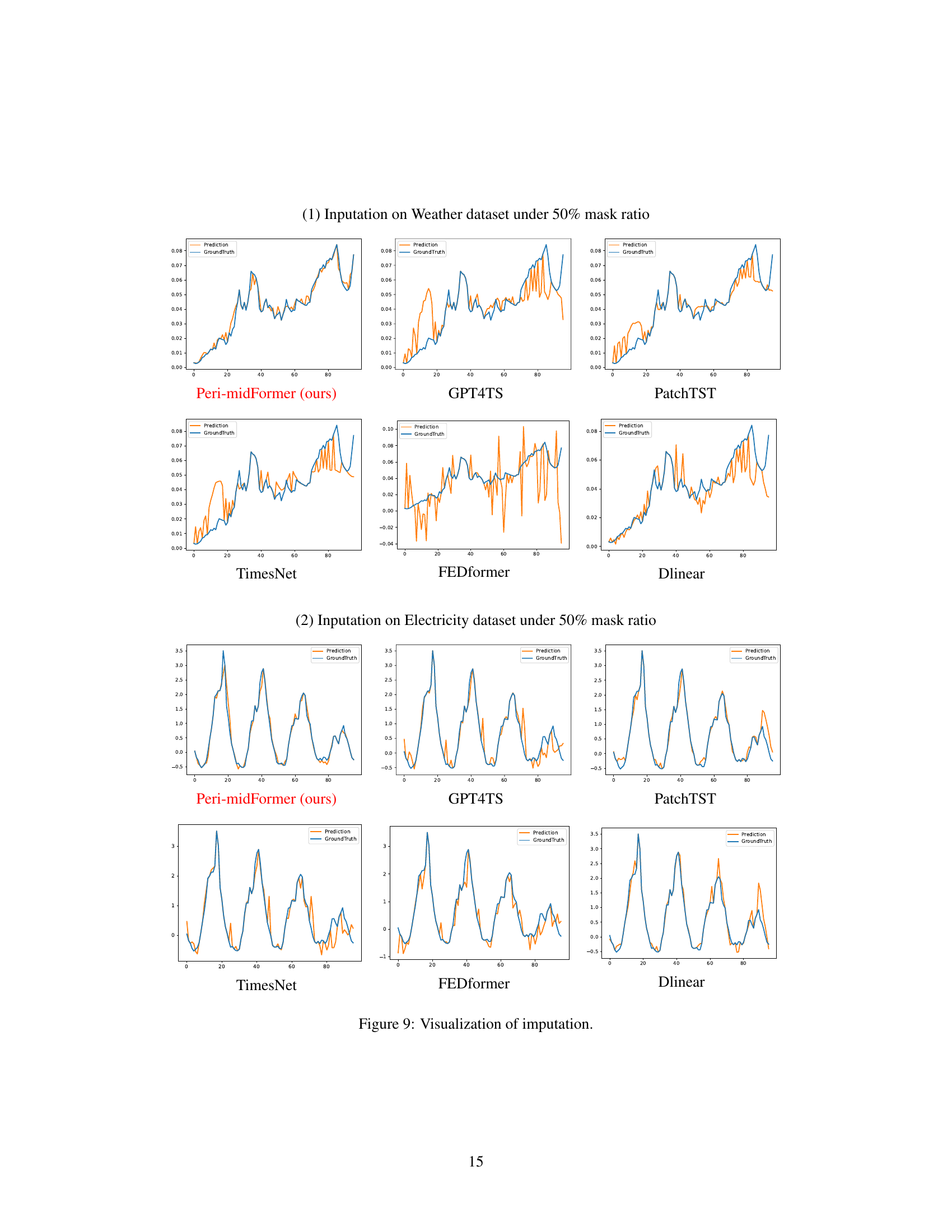
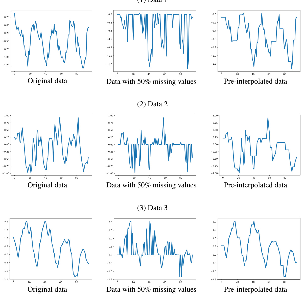
This figure visualizes the imputation results of six different models (Peri-midFormer, GPT4TS, PatchTST, TimesNet, FEDformer, and DLinear) on two datasets (Weather and Electricity) with a 50% mask ratio. For each dataset and model, it shows the ground truth time series and the corresponding predictions. The visualizations allow for a comparison of the different models’ ability to accurately impute missing values in time series data, highlighting the strengths and weaknesses of each approach.

This figure visualizes the imputation results on the Weather and Electricity datasets with a 50% mask ratio. It compares the performance of Peri-midFormer against GPT4TS, PatchTST, TimesNet, FEDformer, and DLinear. Each sub-figure shows the ground truth (blue) and the predicted values (orange) for a specific time series segment.

This figure shows the overall flowchart of the proposed Peri-midformer model. It starts with time embedding of the original time series. Then, it uses the Fast Fourier Transform (FFT) to decompose the time series into multiple periodic components of varying lengths across different levels, forming the Periodic Pyramid. Each component is treated as an independent token and receives positional embedding. The Periodic Pyramid is then fed into the Peri-midFormer, which consists of multiple layers for computing Periodic Pyramid Attention (PPAM). Finally, there are two strategies for downstream tasks: For classification tasks, components are directly concatenated and projected into the category space. For other reconstruction tasks (forecasting, imputation, and anomaly detection), features from different pyramid branches are integrated through Periodic Feature Flows Aggregation to generate the final output.

This figure visualizes the imputation results of different models on the Weather and Electricity datasets. For each dataset, it shows the original data, data with 50% missing values, and the imputation results of Peri-midFormer, GPT4TS, PatchTST, TimesNet, FEDformer, and DLinear. The visualization helps to understand the performance of each model in terms of capturing the underlying patterns of the time series and its ability to reconstruct the missing values.
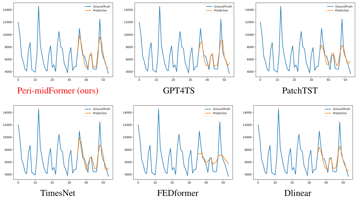
This figure visualizes the imputation results on the Weather and Electricity datasets with a 50% mask ratio. It shows the original ground truth, the imputation results from Peri-midFormer, GPT4TS, PatchTST, TimesNet, FEDformer, and DLinear. The visualizations help to illustrate the relative performance of each method for imputing missing values in time series data.
This figure shows the architecture of the Peri-midFormer model. The input is the original time series, which is first decomposed into multiple periodic components using FFT. These components are organized into a Periodic Pyramid structure, which is then fed into the Peri-midFormer. The Peri-midFormer consists of multiple layers of Periodic Pyramid Attention Mechanism (PPAM), which computes self-attention among periodic components to capture complex temporal variations. Finally, depending on the downstream task, two different strategies are employed: for classification, components are directly concatenated and projected into the category space; for reconstruction tasks (forecasting, imputation, and anomaly detection), features from different pyramid branches are integrated through Periodic Feature Flows Aggregation to generate the final output.
This figure illustrates the architecture of the Peri-midFormer model. The model takes as input the original time series, which is then decomposed into multiple periodic components via FFT. These components are organized into a Periodic Pyramid structure, reflecting their inclusion relationships. Each level in the pyramid contains components with the same period. Positional embeddings are added. The Periodic Pyramid is then fed into the Peri-midFormer which utilizes a Periodic Pyramid Attention Mechanism (PPAM) to capture complex temporal variations among the periodic components across different levels. Finally, depending on the downstream task, two strategies are used: for classification tasks, components are directly concatenated; for reconstruction tasks (such as forecasting and imputation), features are aggregated via Periodic Feature Flows Aggregation before generating the output.

The figure illustrates the inclusion relationships between periodic components at different levels of the Periodic Pyramid (left). It also shows the Periodic Pyramid Attention Mechanism (PPAM) (right) that captures these inclusion and overlap relationships in the attention computation. The left side visually depicts how shorter periods are nested within longer ones. The right side illustrates how PPAM calculates attention not only between components across different pyramid levels but also within the same level, effectively modeling complex temporal relationships within the time series.

The figure shows the inclusion relationships between periodic components. The left panel illustrates how components of different periods overlap and are included within each other, forming a pyramid-like structure. The right panel illustrates the Periodic Pyramid Attention Mechanism (PPAM), which depicts how attention is calculated between periodic components across different levels in the pyramid structure. The arrows indicate the inclusion relationships, where attention is computed among all components within the same level and between components across levels.

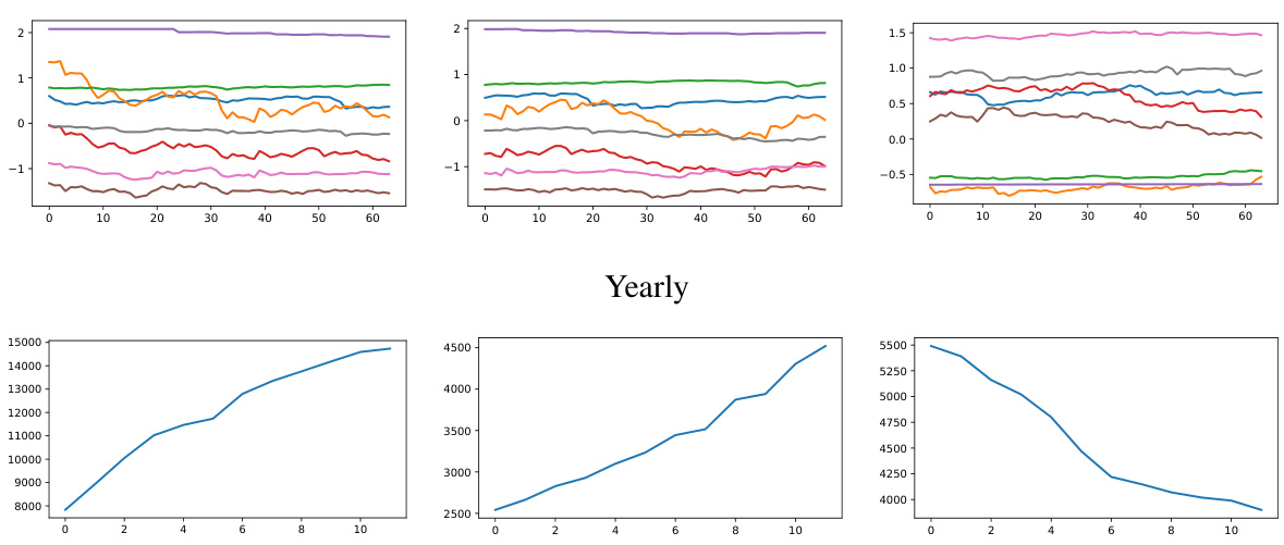
The figure visualizes the pyramid structure of Periodic Feature Flows, where each branch represents a sequence of periodic components from the top to the bottom level of the pyramid. The left panel displays a heatmap showing the number of flows and their dimension (vertical axis), illustrating the structure of the flows and how they are composed of periodic components. The right panel displays the waveform of each feature flow, revealing how the individual feature flows vary in terms of periodic characteristics and their contribution to the overall signal.
This figure illustrates the concept of multi-periodicity in time series, where multiple periodic variations with different periods (e.g., yearly, monthly, weekly, daily) coexist. It shows how these periodic components can be organized hierarchically, with longer periods encompassing shorter periods, forming a pyramid structure. The original time series is at the top of the pyramid, and lower levels represent periodic components with gradually shorter periods. This pyramid structure explicitly represents the inclusion relationships among different levels of periodic components in time series.
This radar chart compares the performance of Peri-midFormer against other state-of-the-art models across five main time series analysis tasks: long-term forecasting, short-term forecasting, imputation, classification, and anomaly detection. Each axis represents a specific task, and the distance from the center indicates the performance (lower is better for MSE, higher is better for accuracy and F1-score). The chart visually demonstrates Peri-midFormer’s consistent superiority across all five tasks.
This figure visualizes the imputation results on the Weather and Electricity datasets with a 50% mask ratio. It compares the imputation performance of Peri-midFormer against several other methods (GPT4TS, PatchTST, TimesNet, FEDformer, and DLinear) by showing the ground truth and predicted values across multiple time series segments. The plots demonstrate how well each model reconstructs the missing data points.
More on tables

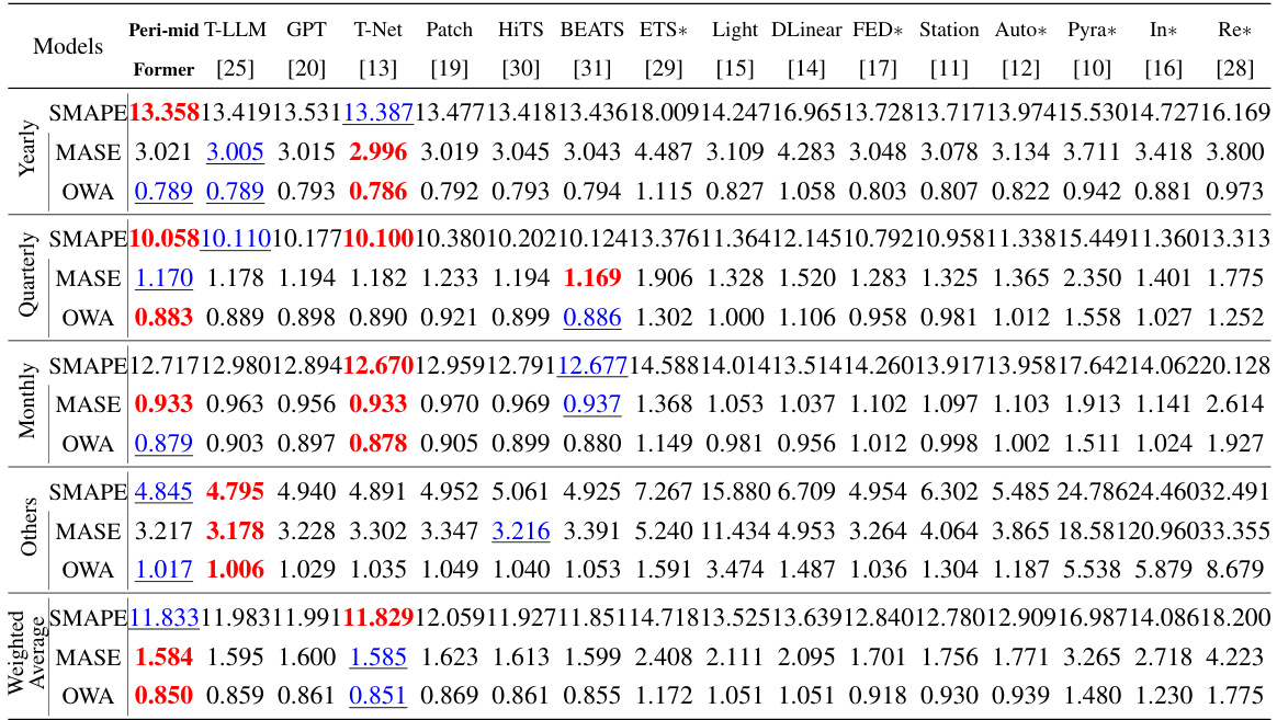
This table presents the results of short-term forecasting experiments on the M4 dataset. It compares the performance of Peri-midFormer against various baseline methods across different prediction lengths (6 and 48). The performance metric used is a weighted average of SMAPE, MASE, and OWA, calculated across multiple datasets with varying sampling intervals. The table highlights Peri-midFormer’s competitive performance and indicates the best and second-best performing models for each metric.

This table presents the results of the imputation task, comparing the performance of Peri-midFormer against other baselines. Different levels of randomly masked data points (12.5%, 25%, 37.5%, and 50%) were used to evaluate the robustness of the methods. The results are averaged over four different mask ratios. The metrics used are Mean Squared Error (MSE) and Mean Absolute Error (MAE). The best and second-best results are highlighted in red and blue, respectively.

This table presents the anomaly detection results on five datasets (SMD, MSL, SMAP, SWaT, and PSM). For each dataset and each model, the table shows the precision (P), recall (R), and F1-score (harmonic mean of precision and recall). Higher values for P, R, and F1 indicate better performance. The table compares the proposed Peri-midFormer to various baselines, highlighting its performance relative to the state-of-the-art.

This table presents the results of long-term forecasting experiments conducted on eight datasets with four different prediction lengths (96, 192, 336, and 720). The results are averaged across these lengths. The table compares the performance of Peri-midFormer against various baselines using the Mean Squared Error (MSE) metric. Red and blue highlight the best and second-best performing methods for each dataset, respectively.
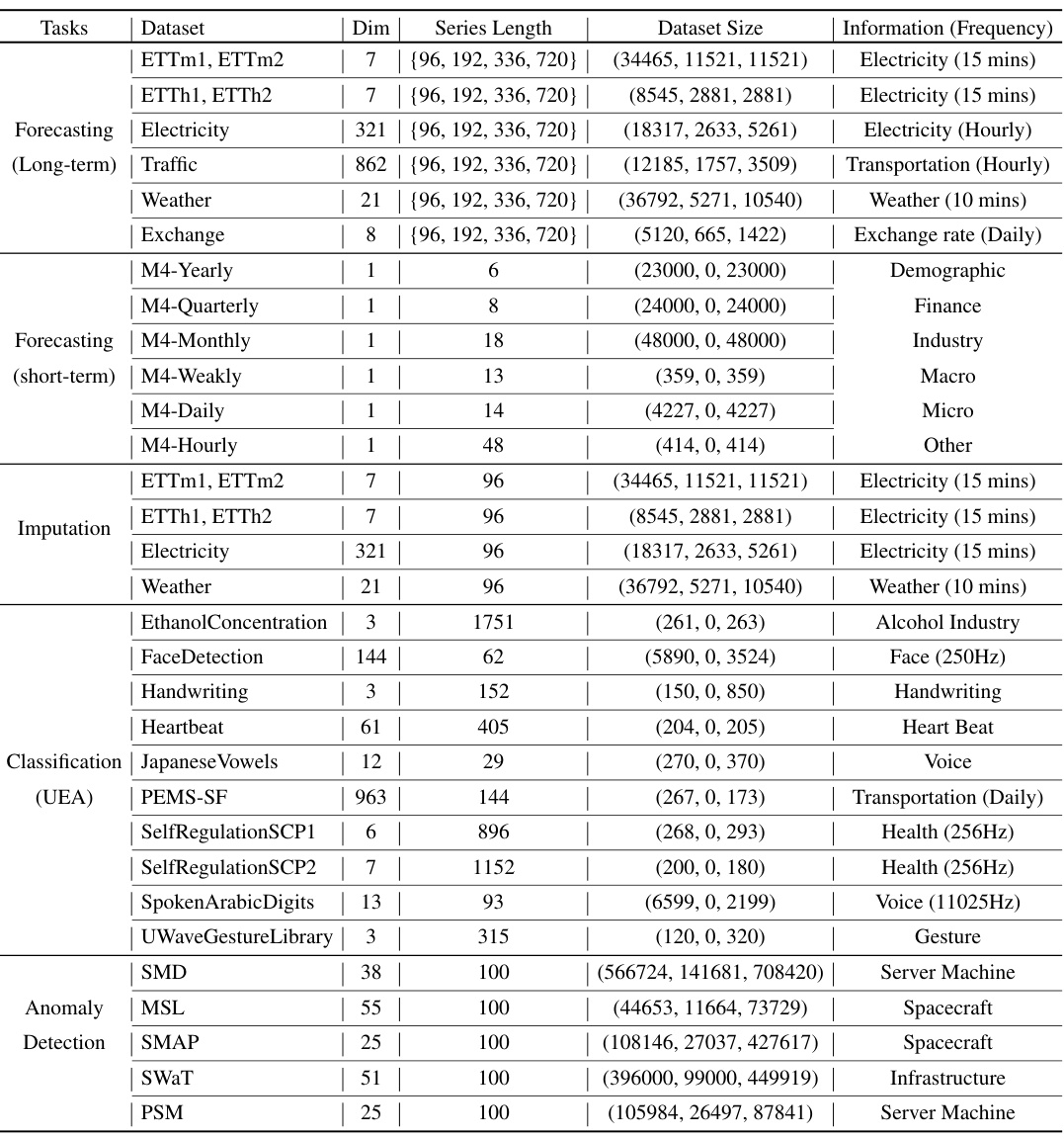
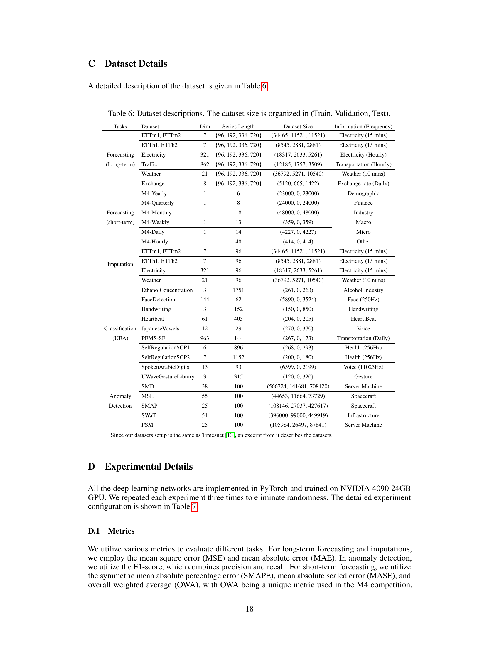
This table provides detailed information about the datasets used in the paper’s experiments. For each dataset, it lists the task it was used for (forecasting, imputation, classification, or anomaly detection), the number of dimensions (Dim), the series length, the dataset size (number of samples in train, validation, and test sets), and a description of the data and its frequency.

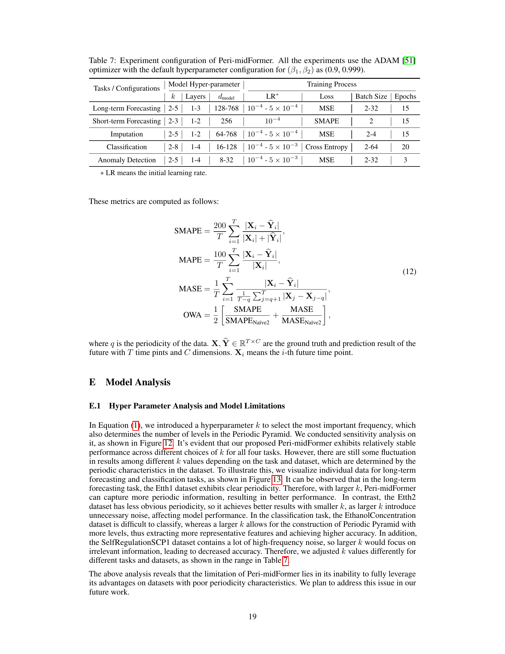
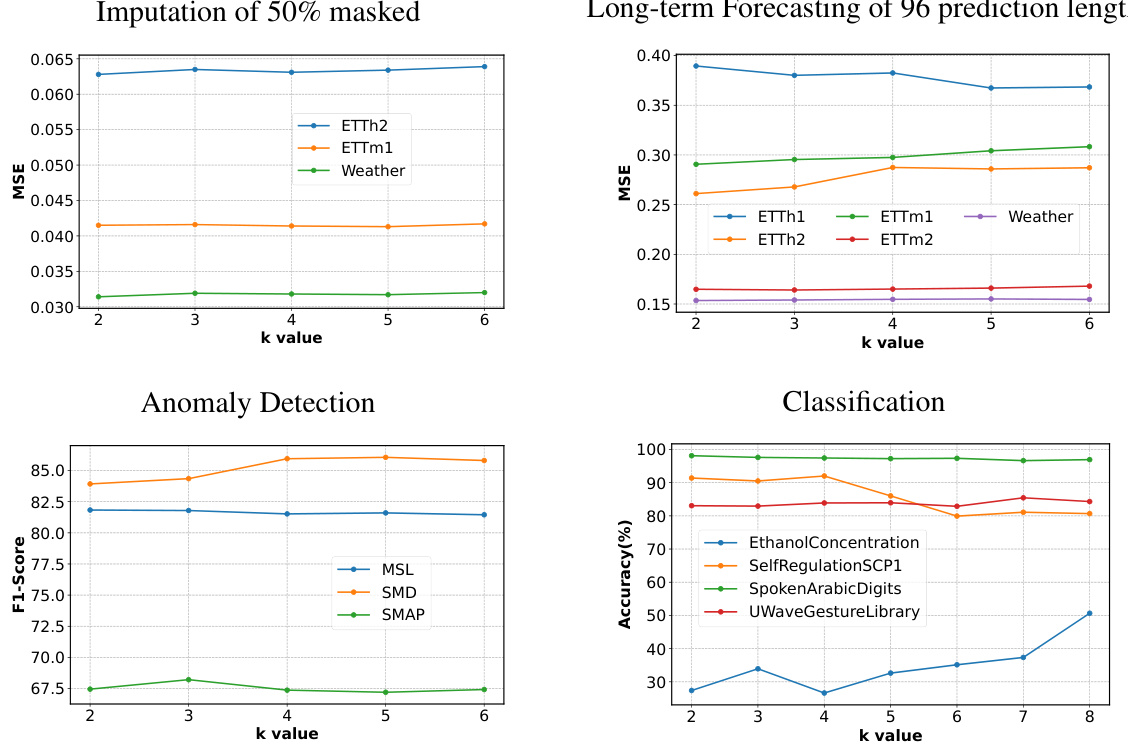
This table details the hyperparameters used in the Peri-midFormer model for each of the five tasks examined in the paper: long-term forecasting, short-term forecasting, imputation, classification, and anomaly detection. It shows the range of values considered for the hyperparameters k, number of layers, dmodel, and learning rate (LR). The loss function, batch size, and number of epochs used during training are also specified for each task.

This table presents the computational cost and time efficiency of different models on the Electricity dataset for long-term forecasting with a prediction length of 720. It compares Peri-midFormer against several baselines, including Time-LLM, GPT4TS, PatchTST, TimesNet, DLinear, and Autoformer. The metrics shown include FLOPS (floating-point operations) for both training and testing, GPU and CPU memory usage during training and testing, training time, testing time per sample, and the Mean Squared Error (MSE). This allows for a comparison of computational efficiency and prediction accuracy across different models.

This table presents the results of complexity and scalability experiments conducted on the Electricity dataset for long-term forecasting with a prediction length of 720. It compares Peri-midFormer against several other methods, showing the training and test FLOPS, GPU and CPU memory usage, training and test times, and the resulting MSE (Mean Squared Error). The table helps to demonstrate the computational efficiency and scalability of Peri-midFormer relative to other approaches.

This table presents the results of ablation experiments conducted to evaluate the impact of pre-interpolation on the imputation task using the ECL dataset. It compares the performance of Peri-midFormer and several baseline models (TimesNet, Pyraformer, DLinear, PatchTST, and ETSformer) with and without pre-interpolation. The results are reported for four different mask ratios (0.125, 0.25, 0.375, and 0.5), indicating varying levels of missing data. The metrics used for evaluation are MSE and MAE.
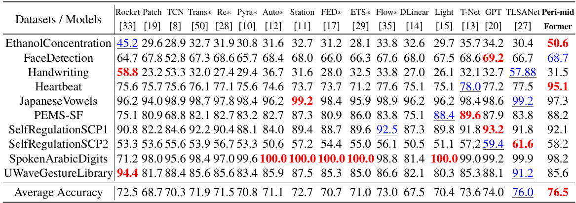
This table presents the classification accuracy achieved by Peri-midFormer and several other baseline methods across ten benchmark datasets from the UEA archive. The table highlights Peri-midFormer’s superior performance compared to other methods. The accuracy scores represent the average across three repetitions of each experiment, with standard deviations within 1%. Note that results for PatchTST and TSLANet were reproduced using publicly available code, while results for other methods were taken directly from the GPT4TS paper.
This table presents the results of the long-term forecasting experiments on eight datasets with four different forecasting lengths. The metrics used to evaluate the performance are Mean Squared Error (MSE) and Mean Absolute Error (MAE). The table shows the average performance across the four forecasting lengths and highlights the best and second-best performing models in red and blue, respectively. More detailed results can be found in Tables 13 and 14.
This table presents the results of long-term forecasting experiments using different models. It compares the performance of Peri-midFormer against several baselines across eight datasets (Weather, ETTh1, ETTh2, ETTm1, ETTm2, Electricity, Traffic, Exchange) with varying prediction lengths (96, 192, 336, 720). The evaluation metrics are Mean Squared Error (MSE) and Mean Absolute Error (MAE). The results are averaged across four prediction lengths, and the best and second-best performances are highlighted.

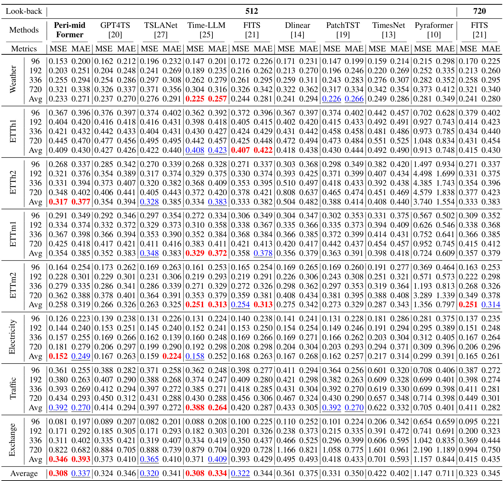
This table presents the performance comparison of Peri-midFormer against other state-of-the-art models on long-term forecasting tasks using a lookback window of 512 time steps. The table shows the mean squared error (MSE) and mean absolute error (MAE) for various datasets and prediction lengths (96, 192, 336, and 720). The best and second-best results are highlighted, indicating Peri-midFormer’s competitive performance. The results for FITS, which uses a lookback window of 720, are also included.

This table presents the results of imputation task on six datasets (ETTm1, ETTm2, ETTh1, ETTh2, Electricity, and Weather) under four mask ratios (12.5%, 25%, 37.5%, and 50%). The results are averaged across all mask ratios. The table compares the performance of Peri-midFormer with other state-of-the-art methods (GPT4TS, TimesNet, PatchTST, ETS*, LightTS, DLinear, FED*, Station, Auto*, Pyra*, In*, and Re*). The metrics used to evaluate the performance are MSE and MAE.

This table presents the results of long-term forecasting experiments conducted on eight real-world benchmark datasets. The models are evaluated using Mean Squared Error (MSE) and Mean Absolute Error (MAE) metrics across four different prediction lengths (96, 192, 336, and 720). The table shows the average performance across these lengths, with the best and second-best results highlighted in red and blue, respectively. Complete results for each prediction length are available in Tables 13 and 14.
Full paper#
