↗ OpenReview ↗ NeurIPS Proc. ↗ Hugging Face ↗ Chat
TL;DR#
Long-term time series forecasting (LTSF) is challenging due to the need to capture long-range dependencies and inherent periodic patterns within data. Existing deep learning models often struggle with efficiency and accuracy in LTSF, particularly when dealing with high-dimensional datasets. This is where CycleNet comes in.
CycleNet tackles these issues by introducing the Residual Cycle Forecasting (RCF) technique. RCF explicitly models periodic patterns using learnable recurrent cycles and then predicts the residual components. Combined with a simple Linear or MLP backbone, CycleNet achieves state-of-the-art accuracy in various domains (electricity, weather, and energy), while being significantly more efficient than other advanced models. This demonstrates that directly modeling periodicity can be highly effective for LTSF tasks.
Key Takeaways#
Why does it matter?#
This paper is significant because it introduces a novel and efficient method for long-term time series forecasting, addressing a crucial challenge in various domains. CycleNet’s superior performance and efficiency advantages make it highly relevant to current research trends in LTSF. The proposed RCF technique, as a plug-and-play module, is highly valuable for enhancing existing models. This research opens up new avenues for further investigations into efficient long-term forecasting techniques.
Visual Insights#
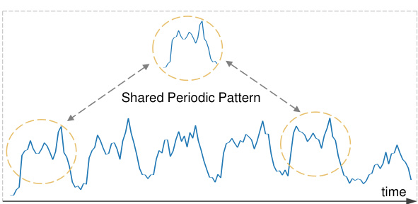
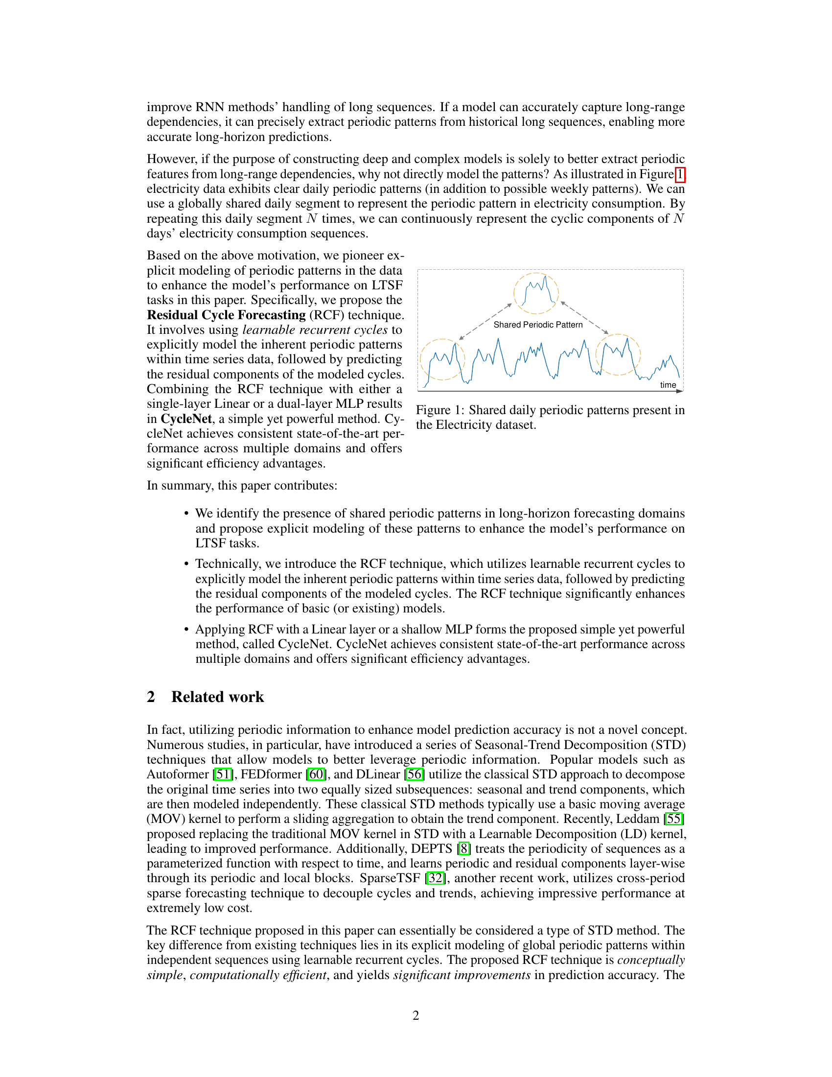
The figure shows that the electricity consumption data exhibits clear daily periodic patterns. A repeating segment representing the daily pattern is highlighted, illustrating the concept of shared periodic patterns that are consistently present in the data over time. This stable periodicity forms the basis for long-term predictions.

This table presents information about the datasets used in the paper’s experiments. It includes the dataset name, the number of timesteps, the number of channels, the frequency of data points (e.g., 1 hour, 15 mins), the types of cyclic patterns observed (Daily, Daily & Weekly), and the length of each cycle.
In-depth insights#
Periodic Pattern Modeling#
The subheading ‘Periodic Pattern Modeling’ likely details a crucial methodology in a time series forecasting research paper. It probably introduces the core concept of explicitly modeling inherent periodic patterns (daily, weekly, seasonal, etc.) within the data, rather than implicitly relying on the model to learn them from long-range dependencies. This approach likely involves using a technique that directly incorporates prior knowledge of the periodic structure of the time series, leading to more accurate and efficient forecasts, especially for long-term forecasting tasks. The method may utilize learnable recurrent cycles, where a repeating pattern is learned and applied to the data. This likely involves generating learned representations for these periodic cycles, potentially as a parameter or component of the forecasting model. The paper likely demonstrates that this explicit modeling improves forecast accuracy compared to relying on purely implicit pattern learning, potentially leading to state-of-the-art results on established benchmark datasets.
RCF Technique#
The Residual Cycle Forecasting (RCF) technique is a novel approach for enhancing time series forecasting by explicitly modeling inherent periodic patterns. Instead of implicitly capturing periodicity through complex model architectures, RCF directly models these patterns using learnable recurrent cycles. This involves generating a set of learnable cycles, which are then cyclically replicated to match the input sequence length. Predictions are performed on the residual components after subtracting the modeled cycles from the original data, effectively isolating the non-periodic elements for improved prediction. This approach offers significant advantages in terms of efficiency, reducing the parameter count drastically compared to existing methods. Furthermore, RCF proves to be a plug-and-play module, seamlessly integrating with existing forecasting models to enhance their performance. The simplicity, computational efficiency, and superior accuracy of RCF make it a promising technique for enhancing long-term forecasting models.
CycleNet Architecture#
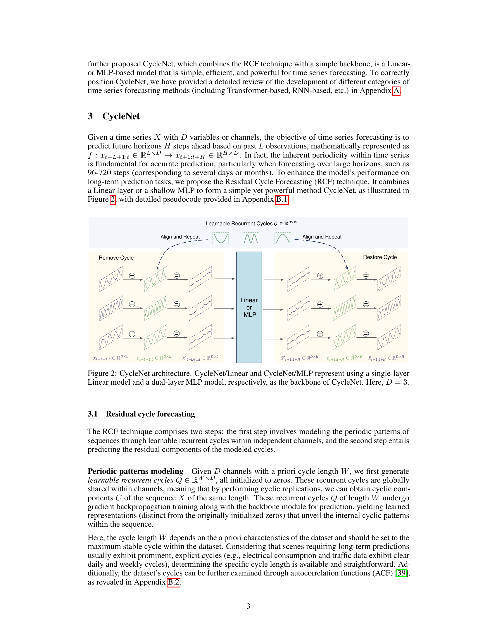
CycleNet’s architecture centers on the novel Residual Cycle Forecasting (RCF) technique. RCF explicitly models inherent periodic patterns within time series data using learnable recurrent cycles. This is a significant departure from methods that implicitly capture periodicity through complex deep learning models. The learned recurrent cycles, represented as a matrix Q, are globally shared across channels. The process involves aligning and repeating these cycles to match the input sequence length, enabling the model to effectively capture cyclic patterns regardless of input length. The cyclical components are then removed from the input, leaving a residual component. A simple backbone (Linear or a shallow MLP) predicts the future residual values. Finally, the predictions are added back to the cyclic components to produce the final forecast, demonstrating an efficient and effective way to integrate explicit periodicity modeling into a time series model. The architecture’s simplicity and modularity are strengths. The plug-and-play nature of RCF also offers the advantage of easily integrating it with other existing time series models.
LTSF Experiments#
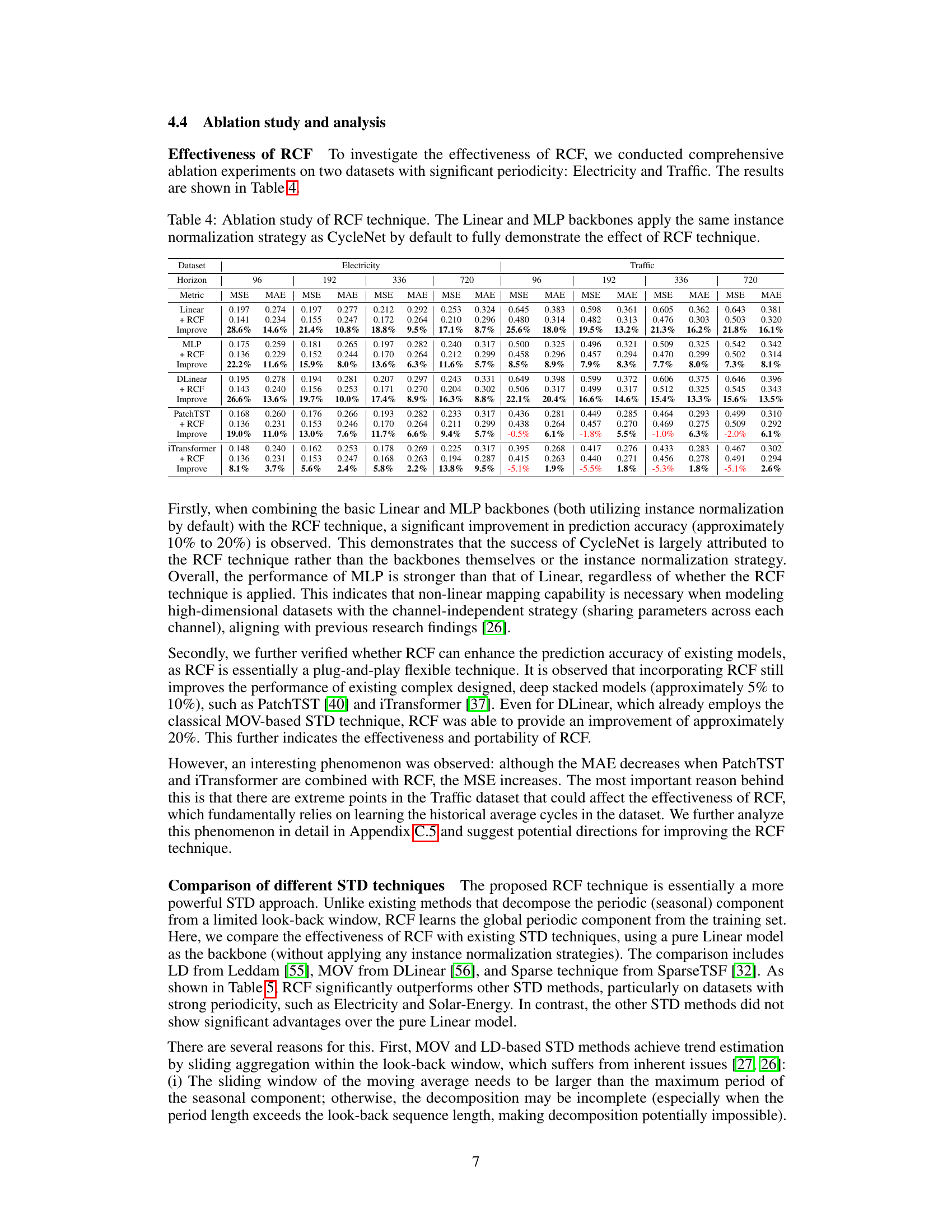
A hypothetical ‘LTSF Experiments’ section would likely detail the empirical evaluation of a long-term time series forecasting (LTSF) model. This would involve selecting diverse and challenging datasets, representative of real-world scenarios. Key aspects would include a rigorous comparison against established baselines, showcasing the proposed model’s superiority across various metrics like Mean Absolute Error (MAE) and Mean Squared Error (MSE). The analysis should explore the model’s performance under different experimental conditions, varying hyperparameters such as lookback window size or forecasting horizon. A thorough ablation study would be crucial, isolating the impact of individual components or design choices. Furthermore, the results should be presented clearly and comprehensively, possibly including tables and visualizations that effectively convey the model’s strengths and limitations in different LTSF tasks. Finally, a discussion of the results’ robustness and generalizability would be essential, addressing potential limitations and suggesting avenues for future research. Statistical significance testing would be critical, ensuring the reported results are not mere chance occurrences.
Future Research#
The paper’s discussion on future research directions highlights several key areas. Extending the RCF technique to handle variable cycle lengths and varying cycle lengths across channels is crucial for broader applicability. The current method assumes consistent periodicity, limiting its effectiveness on datasets with irregular patterns. Addressing this will significantly enhance CycleNet’s robustness. Another important area is improving the model’s handling of outliers and noise. The current approach, while showing strong results, could be made more resilient to noisy data points that can skew the learned periodic patterns. Further research into more sophisticated inter-channel relationship modeling is essential, especially for datasets with strong spatial dependencies like traffic flow. While the paper demonstrates impressive results in several domains, fully exploiting the relationships between channels could significantly improve predictive accuracy. Finally, exploring the potential of applying RCF to long-range periodic patterns (e.g., yearly cycles) is a significant challenge that requires longer historical data and advanced modeling techniques. Success in this area would broaden CycleNet’s utility and impact. Overall, future research should focus on improving the robustness, generalizability, and capacity of CycleNet to better handle complex real-world datasets.
More visual insights#
More on figures

This figure illustrates the architecture of CycleNet, a time series forecasting model. It shows how the model uses learnable recurrent cycles to model periodic patterns in the input time series data. The input data is first processed to remove the cyclic components, leaving only the residual components. These residuals are then passed through a linear layer or a multi-layer perceptron (MLP) to obtain predictions for the residual components. Finally, the predicted residual components are added back to the cyclic components to obtain the final predictions. The figure shows three input channels (D=3) for illustrative purposes.

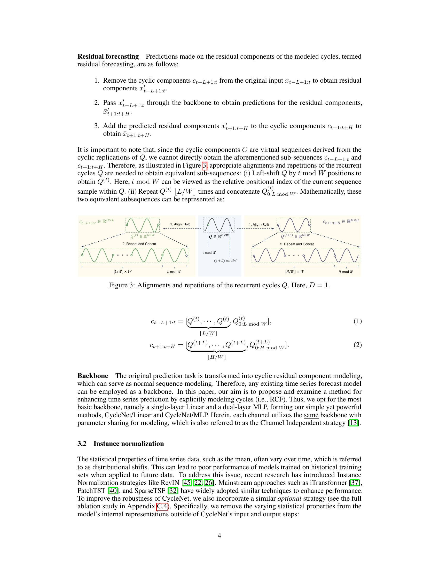
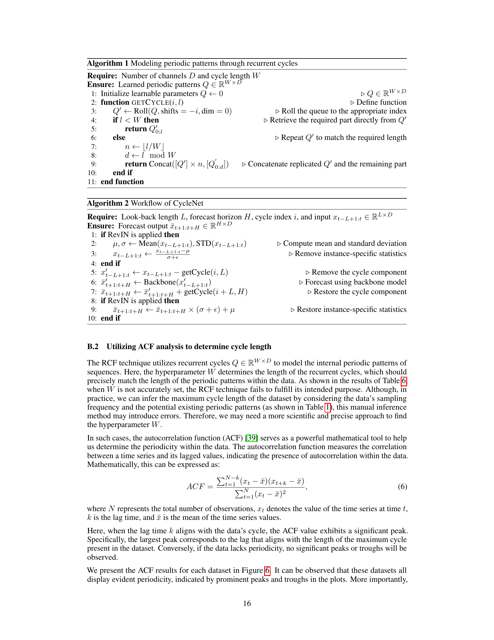
This figure illustrates how the learnable recurrent cycles Q are aligned and repeated to obtain the cyclic components Ct-L+1:t and Ct+1:t+H for the input and output sequences, respectively. The left side shows the input sequence with its cyclic components. The middle shows the process of alignment and repetition of the learnable recurrent cycles Q to generate the cyclic components for the input sequence. The right side shows the process of alignment and repetition of the learnable recurrent cycles Q to generate the cyclic components for the predicted output sequence. The alignment is done by rolling (shifting) Q based on the modulo operation of t and the cycle length W. The repetition is done to match the required length of the subsequence.

This figure illustrates how the recurrent cycles Q are aligned and repeated to obtain the cyclic components C needed for the Residual Cycle Forecasting (RCF) technique in CycleNet. The figure shows that the recurrent cycles Q are first aligned (or rolled) to match the current time step. Then, they are repeated multiple times and concatenated to obtain the desired length of cyclic components to match the input or output length of the model. This process ensures that the cyclic components are correctly aligned with the original time series data.

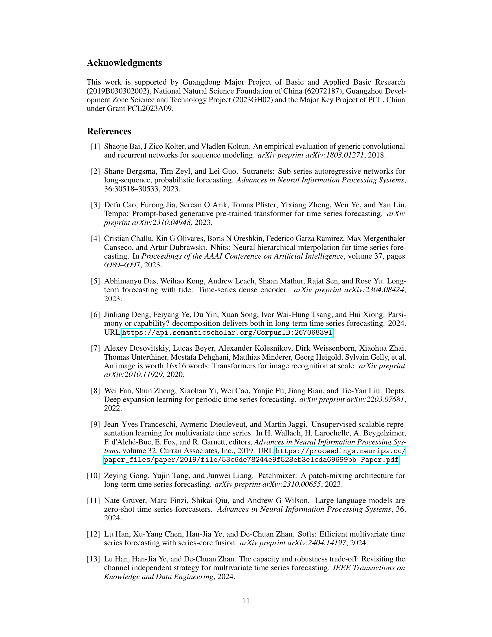
This figure compares the performance of CycleNet against other state-of-the-art models across varying lookback lengths, while maintaining a fixed forecast horizon of 96. It shows how the prediction accuracy (measured by MSE) changes for each model as the amount of historical data used for prediction increases. This allows one to assess the impact of the length of historical data on the effectiveness of each model.

This figure illustrates how the learnable recurrent cycles Q are aligned and repeated to obtain equivalent sub-sequences for the cyclic components in the Residual Cycle Forecasting (RCF) technique. The original input sequence has length L, and the prediction horizon is H. The cycle length is W. The figure shows how the cycles Q are aligned (shifted) based on the current time step (t mod W) and repeated (L/W) or (H/W) times for the input and the prediction, respectively, to create the corresponding cyclic components C for the input and the prediction. This ensures that the model appropriately captures the periodic patterns for the given input sequence and horizon.
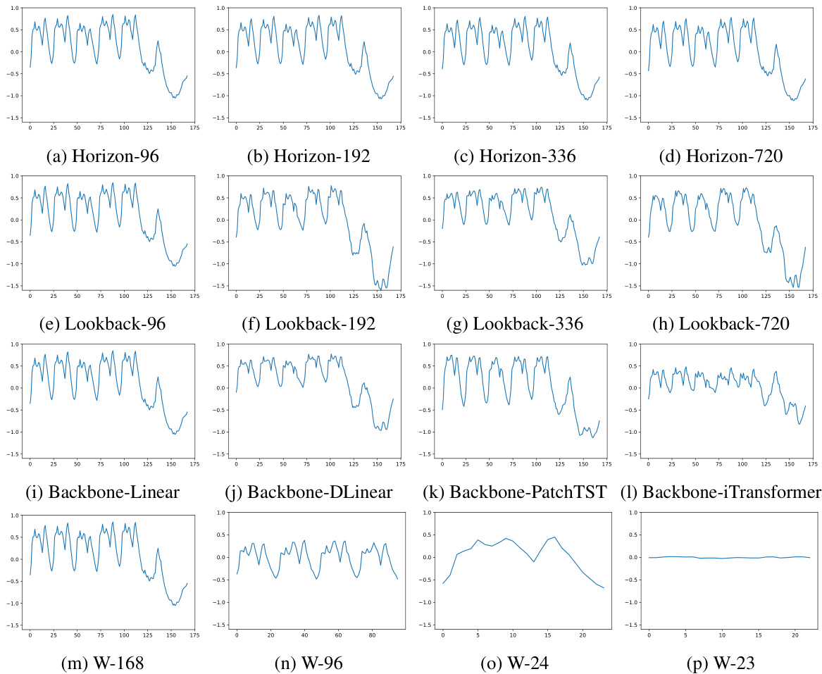
This figure illustrates how the learnable recurrent cycles Q are aligned and repeated to obtain equivalent sub-sequences for the input and output of the backbone. Because the cyclic components C are virtually generated from Q, appropriate alignments and repetitions of Q are needed to match the lengths of the input and output sequences. The figure visually shows how the process is done.
More on tables

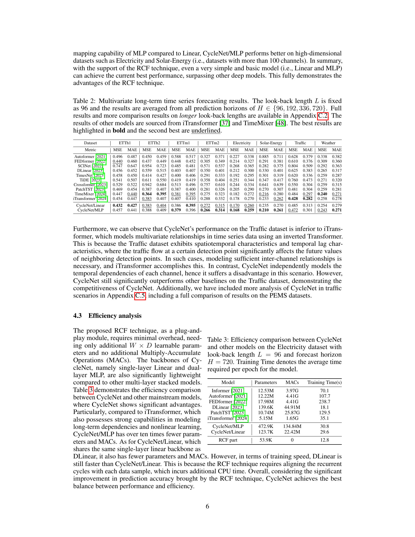
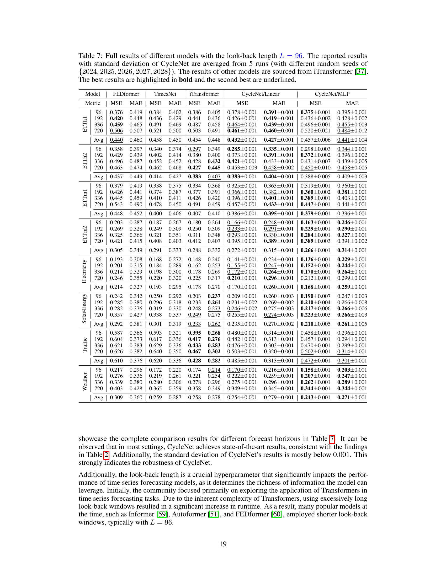
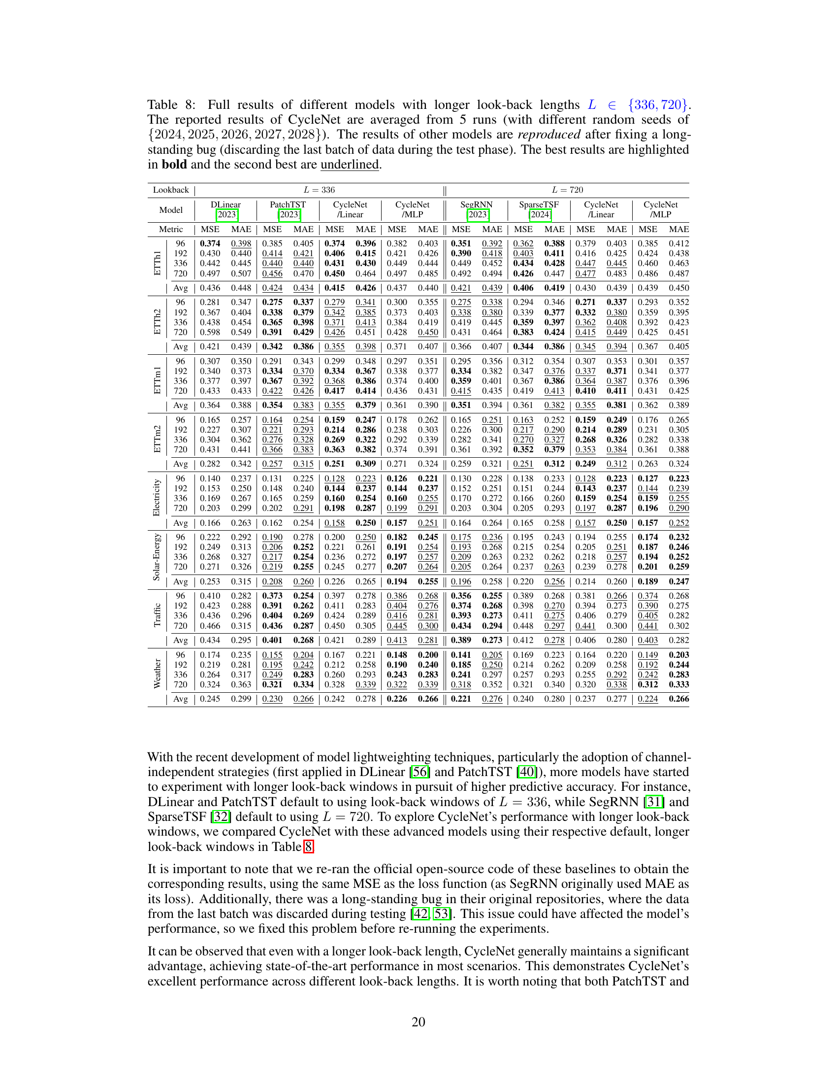
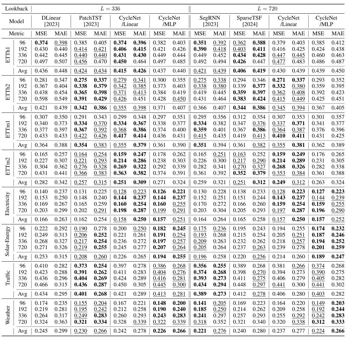
This table presents the main results of the paper, comparing the performance of CycleNet against other state-of-the-art models on multiple long-term time series forecasting tasks. The table shows Mean Squared Error (MSE) and Mean Absolute Error (MAE) metrics, averaged across different prediction horizons, for several benchmark datasets. The best and second-best results are highlighted for clarity.
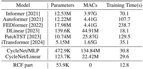
This table compares the efficiency of CycleNet against other state-of-the-art time series forecasting models. The comparison includes the number of parameters, the number of multiply-accumulate operations (MACs), and the average training time per epoch. The results show that CycleNet achieves significant efficiency gains compared to other models while maintaining competitive performance. The RCF component itself introduces minimal computational overhead.
This table presents a comparison of the CycleNet model’s performance against several state-of-the-art time series forecasting models on multiple multivariate datasets. The evaluation metrics used are Mean Squared Error (MSE) and Mean Absolute Error (MAE). The look-back length (L) is consistently set to 96 across all models and datasets. The results shown are averages across multiple prediction horizons (H). The best performing model for each metric and dataset is highlighted in bold, with the second-best underlined. Additional results with longer look-back lengths are available in the appendix.
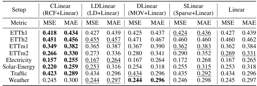
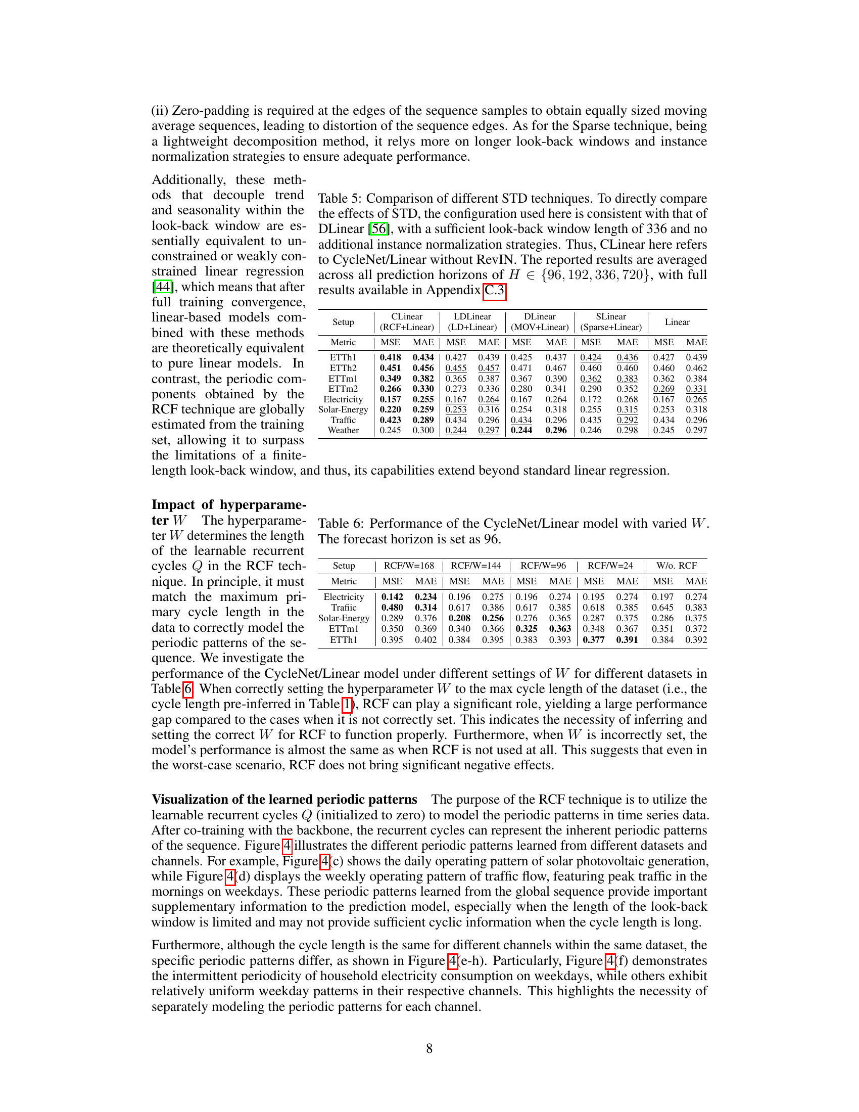
This table compares the performance of CycleNet’s RCF technique against other seasonal-trend decomposition (STD) methods. The experiment uses a simple linear model as a baseline to isolate the impact of the STD method. The results show that RCF outperforms other methods, especially on datasets with strong periodicity, demonstrating its effectiveness in extracting and utilizing periodic patterns for time series forecasting. The table shows MSE and MAE metrics averaged across four different forecast horizons.

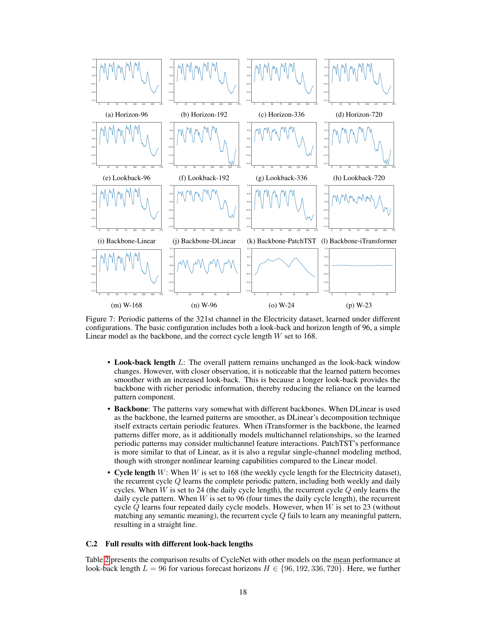
This table shows the performance of the CycleNet/Linear model when the hyperparameter W (cycle length in the RCF technique) is varied. The forecast horizon is fixed at 96. The results are compared for different values of W and also against a model without RCF. This demonstrates the impact of correctly setting the hyperparameter W to match the dataset’s true cycle length for optimal performance. The table highlights that when W is set to the maximum cycle length of the data, RCF significantly improves performance compared to when W is set incorrectly or when RCF is not used at all.

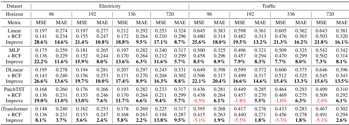
This table presents a comparison of the CycleNet model’s performance against other state-of-the-art time series forecasting models on multiple multivariate datasets. The results are averaged across different prediction horizons (H), using a fixed look-back length (L) of 96. The best and second-best performing models for each metric (MSE and MAE) are highlighted.
This table presents a comparison of the CycleNet model’s performance against other state-of-the-art time series forecasting models on several multivariate datasets. The models are evaluated using Mean Squared Error (MSE) and Mean Absolute Error (MAE) metrics across different prediction horizons (H). The look-back length (L) is fixed at 96 for all models. The best performing model for each metric and dataset is highlighted in bold, while the second-best is underlined. More detailed results with longer look-back lengths are available in the appendix.

This table presents a comparison of the CycleNet model’s performance against several state-of-the-art time series forecasting models on six multivariate datasets (ETTh1, ETTh2, ETTm1, ETTm2, Electricity, Solar-Energy, and Traffic). The results are averaged across different prediction horizons (H) with a fixed lookback length (L=96). The best and second-best performing models for each dataset are highlighted.

This ablation study investigates the impact of instance normalization (RevIN) on CycleNet’s performance. It compares CycleNet with and without RevIN, using both Linear and MLP backbones. The results are presented for various datasets and forecast horizons, illustrating how RevIN contributes to overall performance, although its impact varies across different datasets. The table also includes results from RLinear and RMLP as baselines for comparison.

This table presents the main results of the paper, comparing the performance of CycleNet against other state-of-the-art models on several multivariate long-term time series forecasting datasets. The results are averaged across multiple prediction horizons (H) with a fixed lookback length (L). The best performing model for each metric and dataset is highlighted in bold, and the second-best is underlined.

This table provides details of the datasets used in the paper’s experiments. It lists the name of each dataset, the number of timesteps and channels, the sampling frequency, the type of cyclic patterns present (daily and/or weekly), and the length of these cycles. This information is crucial for understanding the experimental setup and the choice of hyperparameters in the CycleNet model, as the cycle length is used to determine the length of the learnable recurrent cycles.
Full paper#

