↗ OpenReview ↗ NeurIPS Proc. ↗ Chat
TL;DR#
Parameter-Efficient Fine-Tuning (PEFT) methods often struggle with generalization, hindering their performance on unseen data. Existing methods primarily focus on optimizing for specific downstream tasks, sometimes sacrificing the broader knowledge acquired during pre-training. This issue is exacerbated by the fact that naive alignment strategies do not guarantee gradient reduction and can even lead to gradient explosion.
The proposed PACE method addresses these issues by combining parameter-efficient fine-tuning with consistency regularization. By introducing multiplicative noise and ensuring model consistency across perturbations, PACE implicitly regularizes gradients and aligns the fine-tuned model with its pre-trained counterpart. This approach leads to enhanced generalization and superior performance across diverse benchmarks, surpassing existing PEFT methods. Theoretical analysis validates PACE’s effectiveness in achieving both implicit gradient regularization and model alignment.
Key Takeaways#
Why does it matter?#
This paper is crucial for researchers in parameter-efficient fine-tuning (PEFT) because it provides a novel method (PACE) to significantly improve the generalization ability of fine-tuned models, a persistent challenge in the field. PACE’s theoretical framework and superior empirical results across various benchmark datasets offer valuable insights and practical guidance for researchers seeking to enhance the performance and robustness of PEFT methods. The work opens new avenues for investigating efficient and generalizable model adaptation strategies.
Visual Insights#

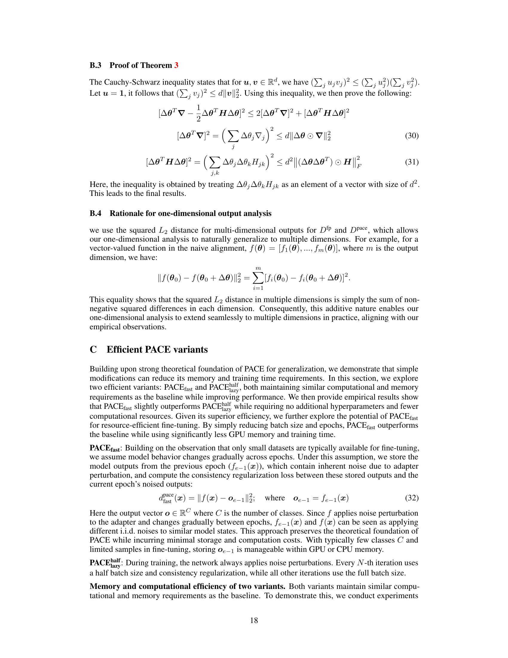
This figure illustrates three theorems of the paper using graphical representations of loss functions. Theorem 1 shows the relationship between flat minima and small gradient and Hessian norms, implying better generalization. Theorem 2 demonstrates how PACE (the proposed method) reduces large differences between perturbed outputs, leading to smaller gradient norms. Theorem 3 shows that PACE implicitly aligns the fine-tuned model with the pre-trained model by minimizing distances between outputs perturbed with different noise, resulting in a reduced FP-distance (Fine-tuned vs Pre-trained distance).
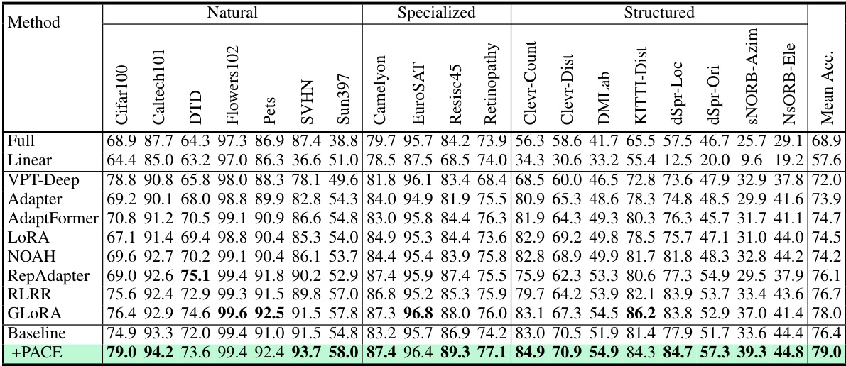
This table presents the results of various parameter-efficient fine-tuning (PEFT) methods on the VTAB-1K benchmark using the ViT-B/16 architecture. It shows the accuracy achieved by each method across different categories of datasets within VTAB-1K, including Natural, Specialized, and Structured images. The ‘Mean Acc.’ column represents the average accuracy across all dataset categories. The table allows for a comparison of PACE against other state-of-the-art PEFT methods to highlight its performance.
In-depth insights#
PEFT Generalization#
Parameter-Efficient Fine-Tuning (PEFT) methods aim to adapt large pre-trained models to downstream tasks efficiently, but often struggle with generalization. A key challenge is balancing task-specific optimization with preserving the knowledge gained during extensive pre-training. Simply minimizing the loss on the target task can lead to overfitting and poor generalization to unseen data. Therefore, research into PEFT generalization focuses on techniques that encourage the fine-tuned model to remain similar to its pre-trained counterpart, thereby retaining beneficial knowledge, while simultaneously adapting to the new task. This often involves strategies like regularization, which constrains the learned parameters, preventing extreme deviations from the pre-trained state. Theoretical analysis often links better generalization with smaller weight gradient norms and larger datasets, providing a framework for developing and analyzing PEFT methods that prioritize generalization.
PACE Regularization#
PACE regularization, as a novel technique, enhances parameter-efficient fine-tuning (PEFT) by implicitly regularizing gradients and aligning the fine-tuned model with its pre-trained counterpart. This dual approach combats the generalization issues often arising from PEFT’s focus on downstream task performance. By introducing multiplicative noise and enforcing consistency across perturbed features, PACE achieves enhanced generalization without significant computational overhead. The theoretical analysis strongly supports the empirical findings, showcasing PACE’s effectiveness across diverse benchmarks. The method’s simplicity and effectiveness make it particularly promising for resource-constrained fine-tuning scenarios.
Gradient Norms#
The concept of ‘gradient norms’ in the context of deep learning, specifically within the framework of parameter-efficient fine-tuning (PEFT), is crucial for understanding model generalization. Smaller gradient norms are theoretically linked to better generalization, as they suggest a flatter minimum in the loss landscape, reducing sensitivity to weight perturbations. The paper investigates this connection, proposing methods to implicitly regularize gradients, thereby enhancing generalization. This is achieved by connecting smaller gradient norms to improved model generalization and aligning the fine-tuned model with its pre-trained counterpart. However, naive alignment doesn’t guarantee gradient reduction, and can even be problematic. The proposed method addresses this challenge by introducing consistency regularization, which implicitly regularizes gradients and enhances alignment. This innovative approach is further supported by theoretical analysis and empirical results demonstrating superior performance on several benchmarks. The study highlights the importance of carefully managing gradients during PEFT to avoid overfitting and ensure robust generalization to unseen data.
PACE Efficiency#
Analyzing PACE’s efficiency requires examining its computational and memory costs relative to its performance gains. PACE introduces additional computational overhead by requiring two passes through the network for consistency regularization. However, efficient variants like PACEfast and PACEhalf mitigate this, achieving comparable performance to the standard PACE with significantly reduced resource consumption. The effectiveness of these variants depends on the dataset size and the trade-off between computational cost and accuracy. Smaller datasets benefit more from these efficient versions. Furthermore, the impact of hyperparameters (λ and σ) needs careful consideration, as their optimal values depend on the specific dataset and task. While PACE requires hyperparameter tuning, the relationship between hyperparameters and dataset size (larger λ and σ for smaller datasets) offers practical guidance. Overall, the efficiency of PACE needs to be evaluated in the context of the specific application and resource constraints. Its performance gains need to outweigh its computational costs to be considered truly efficient.
Future of PACE#
The future of PACE hinges on addressing its limitations and exploring its potential across diverse applications. Improving efficiency is crucial; current methods require double-passing data, increasing computational cost. Future research should focus on optimizing algorithms to reduce this overhead. Expanding application domains beyond visual and text tasks is another key area. PACE’s theoretical grounding suggests broad applicability, opening opportunities in areas like audio, multimodal processing, and reinforcement learning. Theoretical enhancements are also needed; exploring how consistency regularization and gradient penalization interact under different noise models and architectures could unlock greater performance and robustness. Further evaluating PACE’s generalization capability on more challenging and diverse benchmarks is also essential to establish its true potential. Finally, exploring ways to make PACE more user-friendly with better hyperparameter tuning strategies and improved integration with existing PEFT frameworks is needed to facilitate wider adoption.
More visual insights#
More on figures

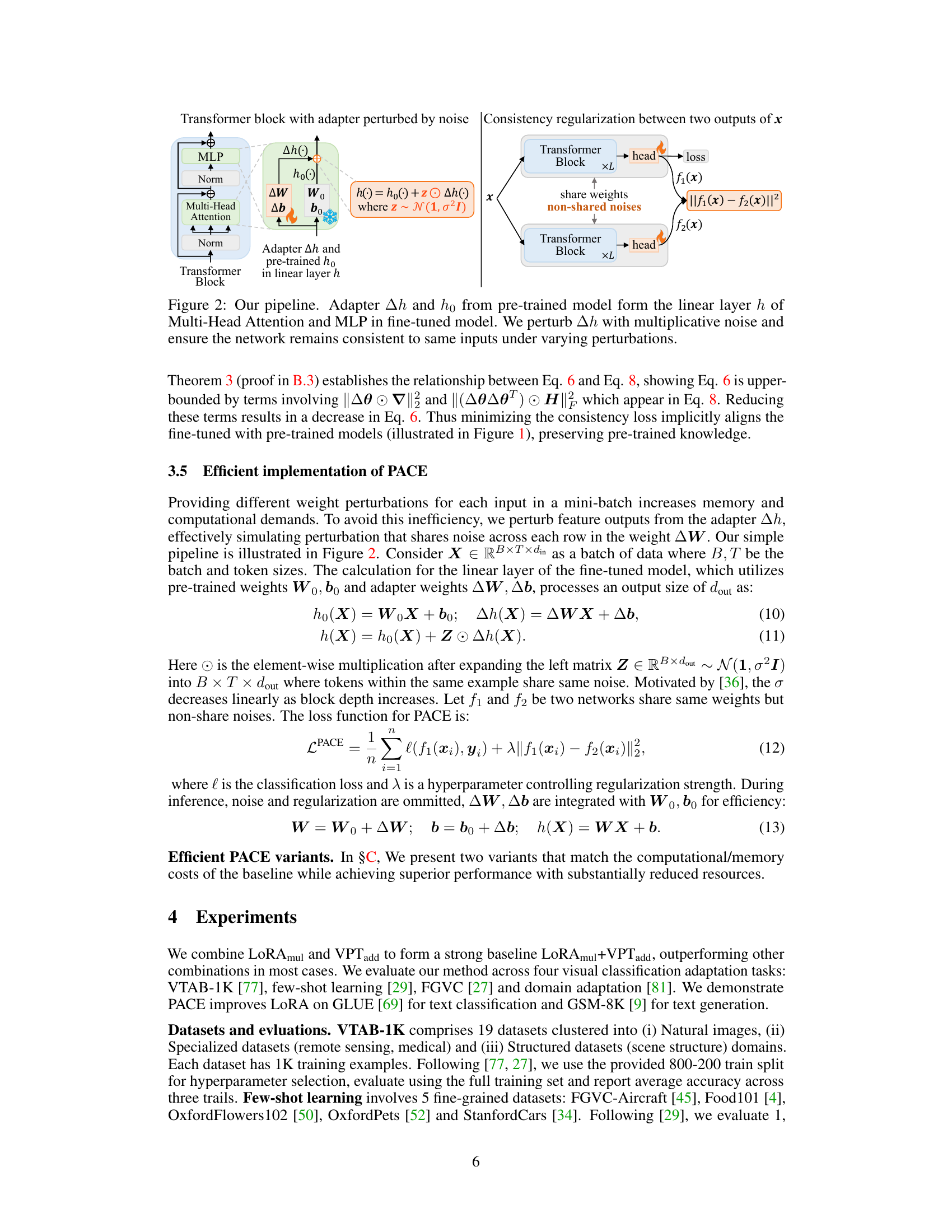
This figure illustrates the PACE pipeline. The pre-trained transformer block (ho) and an adapter (Δh) are combined to form the linear layer (h) in the fine-tuned model. Multiplicative noise (z) is added to the adapter’s output. A consistency regularization loss is applied by comparing the model’s output (f1(x)) with a second model’s output (f2(x)) that uses the same weights but different noise. This forces the model to maintain consistent output across different noise perturbations, thus improving generalization.

This figure presents the results of an analysis comparing the baseline LoRAmul+VPTadd model with the PACE model. The analysis focuses on the validation set of CIFAR-100 from the VTAB-1K benchmark using the ViT-B/16 architecture. Three key metrics are plotted: gradient norm (a), FP-distance (b), and train and validation accuracy (c). Each metric is plotted against training epochs. The figure demonstrates that PACE outperforms the baseline, resulting in lower gradient norms and FP-distances, which correlates to improved generalization performance as evidenced by higher validation accuracy.

This figure shows the results of an experiment comparing the performance of the proposed PACE method against a baseline LoRAmul+VPTadd method. The experiment was conducted on the CIFAR-100 dataset from the VTAB-1K benchmark using a ViT-B/16 model. The figure contains three subplots: (a) shows the gradient norms of both methods during training. (b) shows the FP-distance (output distance between fine-tuned and pre-trained models) for both methods. (c) shows the training and validation accuracy for both methods. The results demonstrate that PACE achieves lower gradient norms and FP-distance, leading to better generalization performance as indicated by higher validation accuracy, compared to the baseline.

The figure shows the gradient norms of different models trained with various regularization strengths (λ) on the CIFAR-100 dataset using the ViT-B/16 model. It demonstrates how the proposed PACE method effectively controls gradient norms across a wide range of λ values, unlike the naive alignment approach (FPA) which exhibits unpredictable behavior and may even lead to gradient explosion. The plot highlights PACE’s robust gradient regularization capability, essential for improved generalization.
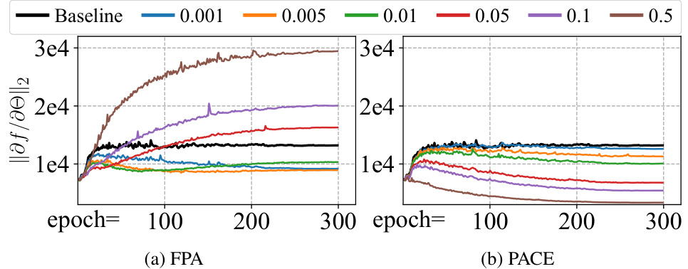
This figure shows the experimental results of applying PACE on the CIFAR-100 dataset of the VTAB-1K benchmark using the ViT-B/16 model. Three subplots are presented. Subplot (a) displays the gradient norm over training epochs for both the baseline LoRAmul+VPTadd and PACE methods. Subplot (b) shows the FP-distance (output distance between fine-tuned and pre-trained models) over epochs. Subplot (c) illustrates the training and validation accuracy for both methods over epochs. The results demonstrate that PACE reduces the gradient norm and maintains a lower FP-distance than the baseline while achieving higher validation accuracy.

This figure shows the gradient norms of different models trained with varying regularization strengths (λ) on the CIFAR-100 dataset using the ViT-B/16 architecture. The baseline model is compared against models using Fine-tuned Pre-trained model Alignment (FPA) and PACE. The plot demonstrates how PACE consistently reduces gradient norms across a wide range of λ values, while FPA shows unpredictable behavior and even gradient explosion in certain regions. The shaded areas represent the standard deviations of the gradient norms across different training epochs. The results visually support the theoretical findings of the paper, highlighting the effectiveness of PACE in gradient regularization.
More on tables
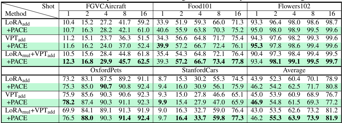
This table presents the classification accuracy results for few-shot learning experiments using a ViT-B/16 model pre-trained on ImageNet-21K. The results are broken down by the number of shots (1, 2, 4, 8, 16) and across five different fine-grained image datasets: FGVC-Aircraft, Food101, OxfordFlowers102, OxfordPets, and StanfordCars. The table compares the performance of the baseline LoRAmul+VPTadd method with and without the PACE enhancement. It shows the average accuracy across these datasets as well. The table helps demonstrate PACE’s effectiveness in improving few-shot learning performance.
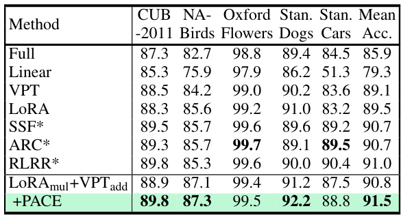
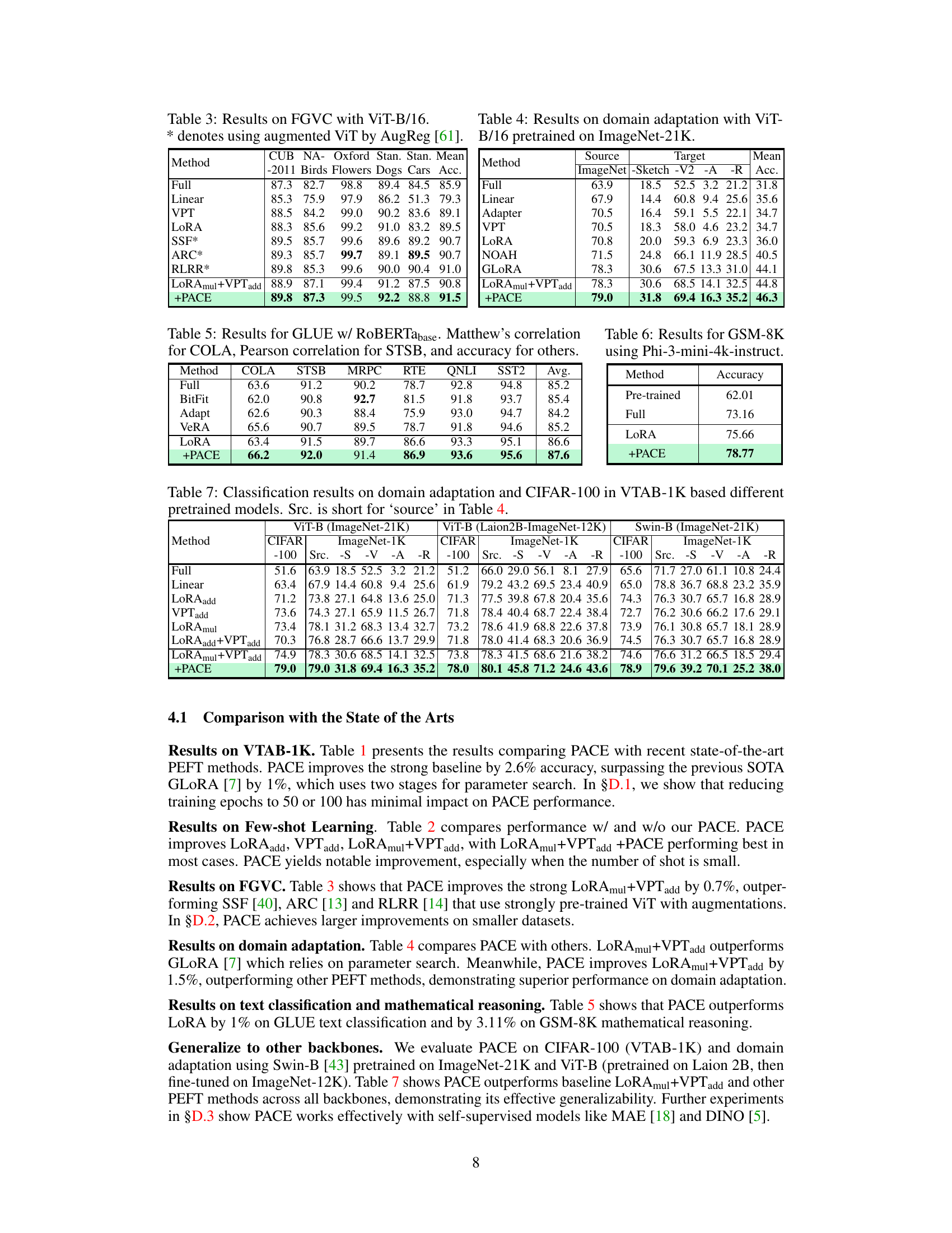
This table presents the results of experiments conducted on the FGVC benchmark using the ViT-B/16 model. It compares the performance of various methods, including a baseline and the proposed PACE method, across five fine-grained datasets: CUB-200-2011, NABirds, Oxford Flowers, Stanford Dogs, and Stanford Cars. The results show the classification accuracy achieved by each method on each dataset. The asterisk (*) indicates that the method used augmented ViT as described in AugReg [61].
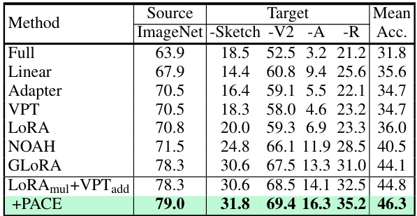
This table presents the results of domain adaptation experiments using the ViT-B/16 model pretrained on ImageNet-21K. The model is evaluated on its performance on ImageNet-Sketch, ImageNet-V2, ImageNet-A, and ImageNet-R datasets. The results are compared across various parameter-efficient fine-tuning (PEFT) methods, including Full fine-tuning, Linear probing, Adapter, VPT, LoRA, NOAH, GLORA, LoRAmul+VPTadd, and the proposed PACE method. The table shows that PACE improves upon the best-performing baseline (LoRAmul+VPTadd) in terms of mean accuracy across all target datasets, demonstrating its effectiveness in domain adaptation.

This table presents the results of experiments conducted on the GLUE benchmark using the ROBERTabase model. It shows the performance of various methods (Full, BitFit, Adapt, VeRA, LoRA, and PACE) across six different GLUE tasks: COLA, STSB, MRPC, RTE, QNLI, and SST2. The metrics used are Matthew’s correlation coefficient for COLA, Pearson correlation coefficient for STSB, and accuracy for the remaining tasks. The table highlights the improvement achieved by adding PACE to the LoRA model, resulting in better overall performance on the GLUE benchmark.

This table presents the classification accuracy results on the GSM-8K benchmark for different fine-tuning methods. The results are shown for the pre-trained model, a fully fine-tuned model, LoRA, and LoRA with PACE. It demonstrates the performance improvement achieved by PACE in comparison to other methods on this mathematical reasoning task.

This table presents a comparison of classification accuracy across various methods (full finetuning, linear probing, different PEFT methods, and PACE) on the CIFAR-100 dataset and domain adaptation tasks within the VTAB-1K benchmark. The results are categorized by different pretrained models (ViT-B with ImageNet-21K weights, ViT-B with Laion2B-ImageNet-12K weights, and Swin-B with ImageNet-21K weights). The source dataset is specified, along with results on various target datasets (ImageNet-Sketch, ImageNet-V2, ImageNet-A, and ImageNet-R). It helps to evaluate the generalization performance and effectiveness of different fine-tuning approaches across different pretrained models.
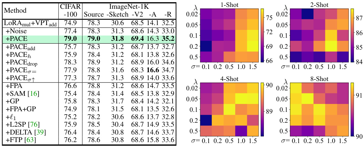
This table presents classification accuracy results on domain adaptation and CIFAR-100 tasks, using the VTAB-1K benchmark. It compares the performance of different pre-trained models (ViT-B with ImageNet-21K weights, ViT-B with Laion2B-ImageNet-12K weights, and Swin-B with ImageNet-21K weights) and fine-tuning methods (Full, Linear, LoRAadd, VPTadd, LoRAmul, LoRAmul+VPTadd, and PACE). The results are broken down by dataset (CIFAR-100 and ImageNet-1K) and target domain (Source, Sketch, V2, A, R). The table highlights the improved performance of PACE compared to other methods.

This table compares the maximum GPU memory usage, total training time and accuracy of different methods on three datasets: CIFAR-100, Camelyon, and ImageNet. The methods compared include the baseline LoRAmul+VPTadd and several variants of PACE, including PACEfast and PACEhalf with different values of N. The results show that PACEfast and PACEhalf achieve similar or better accuracy than the baseline while using significantly less GPU memory and training time.

This table compares the additional memory needed by PACEfast with the baseline GPU memory usage for three different tasks: CIFAR-100 (VTAB-1K), Camelyon (VTAB-1K), and ImageNet (Domain adaptation). It shows that the memory overhead of PACEfast is insignificant compared to the baseline, ranging from 0.0042% to 0.67%. This demonstrates the efficiency of PACEfast in terms of memory usage.

This table presents the results of experiments conducted using PACEfast with reduced batch size and epochs on three different datasets: CIFAR-100, Camelyon, and ImageNet. Each dataset was processed using a different backbone model (ViT-16/B or Swin-B) and the results show significant improvements in memory efficiency and training time compared to the baseline while maintaining superior accuracy.

This table presents classification accuracy results on the VTAB-1K benchmark using various methods and different training epochs (50, 100, 200, 300, and 530). The results are categorized by dataset group (Natural, Specialized, and Structured) and show the average accuracy across the groups. It demonstrates how the performance of different methods varies with the number of training epochs.

This table presents the classification accuracy results on five fine-grained visual categorization datasets (FGVC) using the ViT-B/16 model. The results are shown for different training data sizes, namely 50%, 20%, and 10% of the original training data. The table compares the performance of the baseline LoRAmul+VPTadd method with the proposed PACE method across all five datasets at these varying data sizes. It demonstrates the ability of PACE to maintain and even improve performance under data scarcity, aligning with the paper’s theoretical analyses about better generalization with smaller gradient norms and larger datasets.

This table presents the classification accuracy results on four VTAB-1K sub-datasets (SVHN, Camelyon, Clevr-Count, Clevr-Dist) using different methods. The results are broken down by whether the ViT-16/B model was fully fine-tuned, only linearly probed, fine-tuned using LoRAmul+VPTadd, or fine-tuned using LoRAmul+VPTadd with the proposed PACE method. The models were pre-trained using either self-supervised DINO or MAE methods on the ImageNet-1K dataset. The table demonstrates the performance improvements achieved by using PACE in self-supervised scenarios.

This table compares the performance of various parameter-efficient fine-tuning (PEFT) methods, both with and without the proposed PACE method, on two tasks: CIFAR-100 (from the VTAB-1K benchmark) and ImageNet domain adaptation. It shows the average accuracy across multiple source and target datasets for domain adaptation, highlighting the performance improvement achieved by incorporating PACE into existing PEFT methods such as AdaptFormer, GLORA, COFT, and BOFT.

This table shows the hyperparameter settings used for the baseline models (LoRAmul+VPTadd and LoRAadd) on the VTAB-1K benchmark using the ViT-B/16 architecture. It specifies the rank, learning rate, and weight decay for each of the 19 datasets in VTAB-1K, categorized into Natural, Specialized, and Structured sets. The table also indicates which baseline model (A or B) these hyperparameters are for, enabling a better understanding of model variations across different datasets.

This table presents the classification accuracy results for different few-shot learning scenarios using the ViT-B/16 model pretrained on ImageNet-21K. It compares the performance of different methods (LoRAadd, VPTadd, and LoRAmul+VPTadd) with and without the PACE technique. The results are broken down by the number of shots (1, 2, 4, 8, 16) and across five fine-grained datasets (FGVC-Aircraft, Food101, OxfordFlowers102, OxfordPets, and StanfordCars). The ‘Average’ column shows the average accuracy across all datasets for each method and shot number.

This table lists the hyperparameters used for the LoRAmul+VPTadd baseline model in the FGVC (Fine-Grained Visual Categorization) experiments. It shows the learning rate, weight decay, and rank used for each of the five fine-grained datasets included in the FGVC benchmark: CUB-200-2011, NABirds, OxfordFlowers, StanfordDogs, and StanfordCars. The ‘Mean Parameter (M)’ column indicates the average number of trainable parameters across all datasets for this baseline configuration.

This table shows the hyperparameter settings used for the LoRAmul+VPTadd baseline model in the domain adaptation experiments. It includes the rank, learning rate, and weight decay values used for different tasks, along with the total number of trainable parameters (in millions). These settings were determined through a process of grid search to optimize performance.
Full paper#
