↗ OpenReview ↗ NeurIPS Proc. ↗ Chat
TL;DR#
Solving large-scale sparse linear systems is computationally expensive, especially for those with poor conditioning. Traditional Krylov subspace methods, though widely used, often suffer from slow convergence. This research addresses the issue by exploring data-driven approaches to improve efficiency.
The proposed method, NeurKItt, uses a neural network to predict the invariant subspace of the linear system and integrates this prediction into the Krylov iteration process. This approach significantly reduces the number of iterations needed to achieve the solution, resulting in notable speedups across various datasets and problem settings. The authors demonstrate the feasibility and effectiveness through both theoretical analysis and extensive experiments, showcasing its potential to significantly improve the efficiency of linear system solvers.
Key Takeaways#
Why does it matter?#
This paper is crucial for researchers working on large-scale linear system solving, a fundamental problem across numerous scientific and engineering disciplines. The proposed Neural Krylov Iteration (NeurKItt) offers a significant advancement by accelerating the process, leading to faster computations and improved efficiency. This opens new avenues for tackling computationally demanding problems, making it relevant to current research trends in scientific computing and machine learning.
Visual Insights#

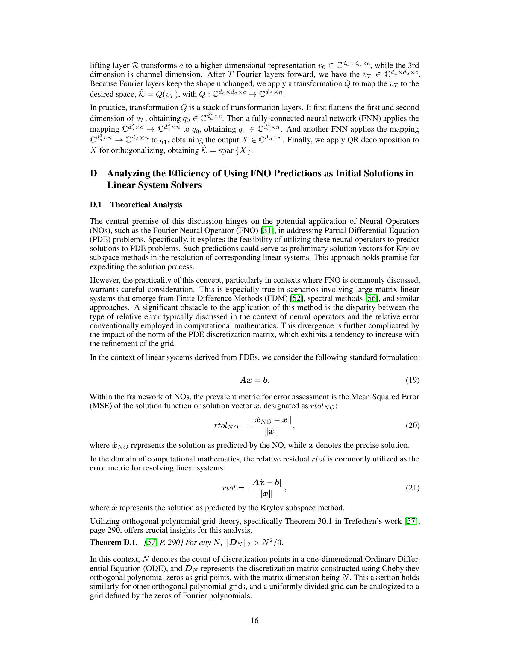
This figure compares the performance of NeurKItt and GMRES in solving linear systems across various preconditioning techniques. Each line shows the convergence of one method with a particular preconditioner. NeurKItt demonstrates significantly faster convergence than GMRES in terms of both time (left panel) and number of iterations (right panel), achieving speedups of up to 5.5x and 16.1x, respectively. This highlights NeurKItt’s ability to accelerate the solving process.
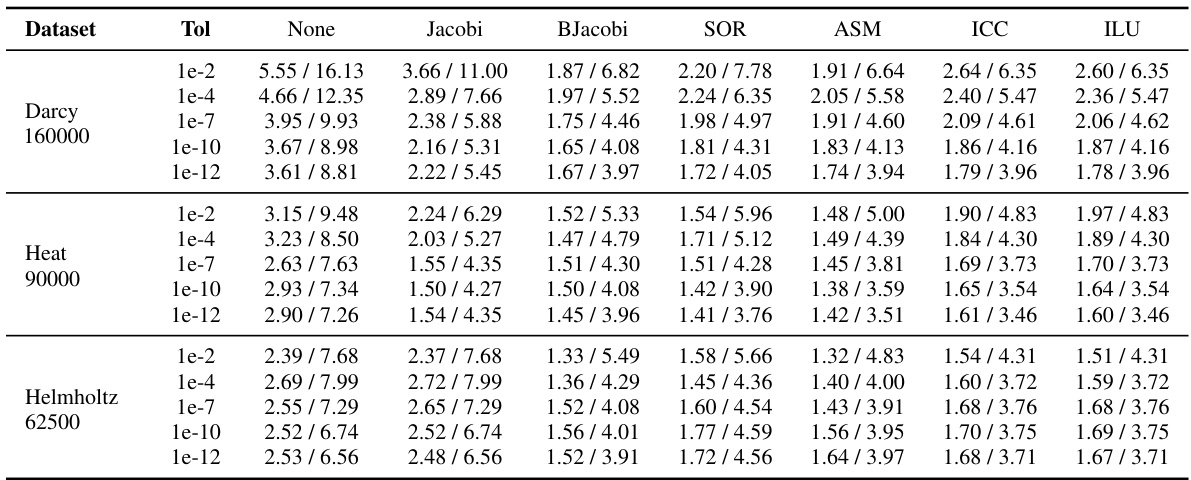
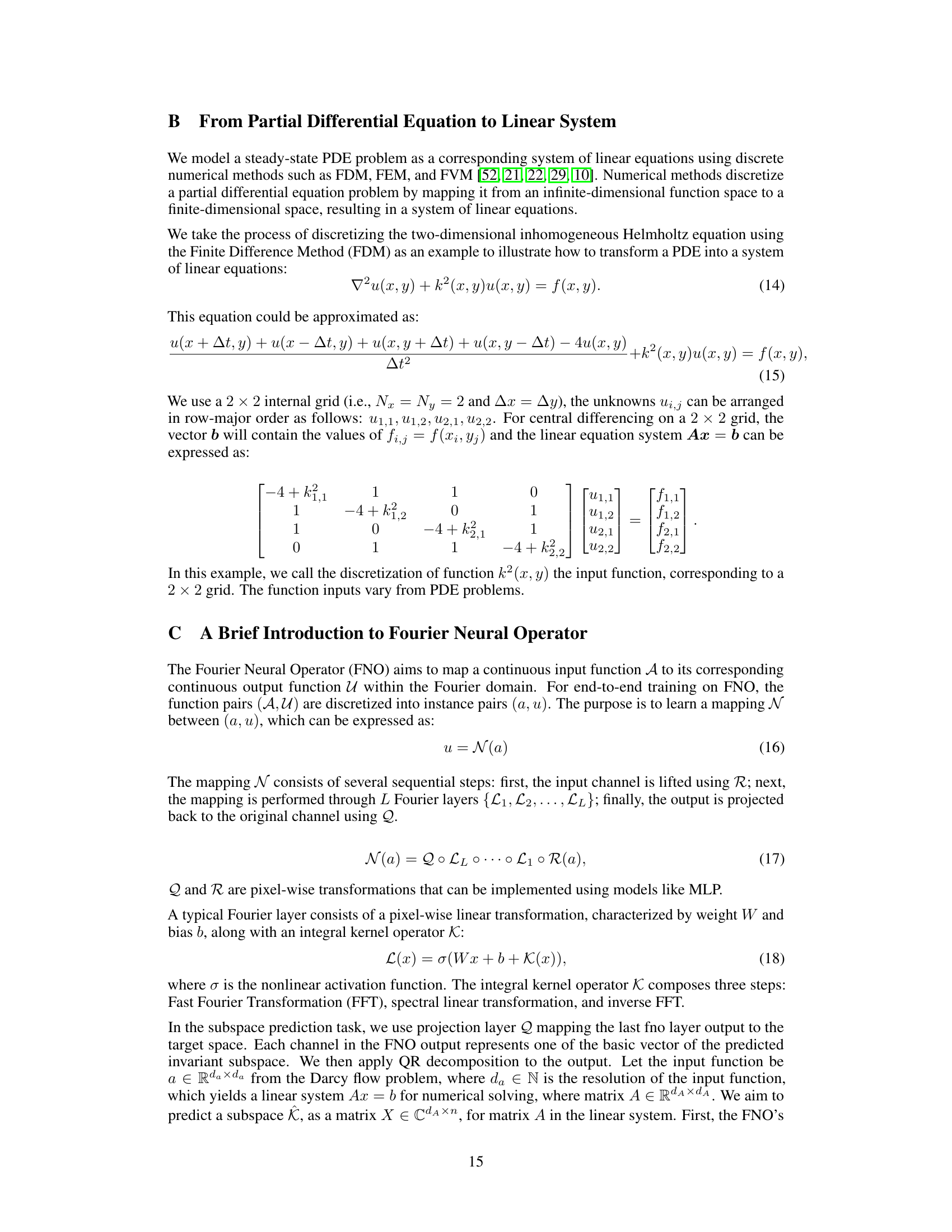
This table compares the performance of NeurKItt and GMRES in solving linear systems. It shows the time and iteration speedup of NeurKItt over GMRES for various datasets (Darcy, Heat, Helmholtz), preconditioning methods (None, Jacobi, BJacobi, SOR, ASM, ICC, ILU), and tolerance levels (1e-2 to 1e-12). Each cell presents the speedup in computation time and the speedup in the number of iterations. The results demonstrate NeurKItt’s efficiency improvements across diverse settings.
In-depth insights#
NeurKItt: Core Idea#
NeurKItt’s core idea centers on accelerating Krylov subspace iterative methods for solving linear systems by leveraging a neural network to predict the system’s invariant subspace. Instead of starting Krylov iterations from a random vector, NeurKItt uses this predicted subspace as a warm start. This significantly reduces the number of iterations needed for convergence, thereby improving both computational speed and stability. The neural operator within NeurKItt predicts the invariant subspace, acting as a data-driven preconditioning technique. By guiding the iterative process with prior knowledge of the subspace, NeurKItt effectively bypasses the less-than-ideal initial iterations that plague traditional Krylov solvers. This approach is particularly beneficial for large-scale sparse linear systems, common in scientific computing. The key novelty lies in the intelligent combination of neural operators and established Krylov methods, creating a hybrid approach that benefits from both data-driven efficiency and well-understood iterative techniques. QR decomposition further enhances subspace prediction accuracy.
Subspace Prediction#
The core of the proposed Neural Krylov Iteration (NeurKItt) method lies in its subspace prediction module. This module leverages neural operators, specifically the Fourier Neural Operator (FNO), to learn a mapping from the input linear system’s characteristics (represented by the matrix A and possibly other relevant parameters) to its invariant subspace K. This prediction is crucial because identifying the invariant subspace allows NeurKItt to accelerate the Krylov subspace iteration by providing a more informed starting point than a random initial vector. QR decomposition is applied to the neural operator’s output to ensure orthogonality and numerical stability of the predicted subspace. The effectiveness of this prediction is demonstrated by a novel projection loss function, specifically designed to minimize the distance between the predicted and true invariant subspaces, optimizing the neural network’s training. This innovative approach enables NeurKItt to significantly reduce the number of iterations needed to solve the linear system, resulting in improved efficiency.
Acceleration Module#
The Acceleration Module in this neural Krylov subspace iteration method is crucial for leveraging the predicted invariant subspace to enhance the Krylov subspace iterative process. It directly incorporates the predicted subspace (K) from the Subspace Prediction Module into the Krylov iteration algorithm, acting as a deflation space. This deflation significantly reduces the dimensionality of the Krylov subspace. The core idea is to cleverly guide the iteration process, effectively warm-starting it by providing the initial subspace. The core algorithm leverages the property that the Krylov subspace iteration approximates the linear system’s invariant subspace. By using this knowledge to refine the process, fewer iterations are required to achieve the desired solution accuracy, leading to substantial computational savings and faster convergence. This module’s effectiveness hinges on the accuracy of the predicted subspace, underlining the importance of the neural operator in the preceding module. The integration of the predicted subspace within the traditional Krylov algorithm is the heart of the acceleration, transforming a time-consuming random-start process into a directed and more efficient approach.
Convergence Analysis#
A rigorous convergence analysis is crucial for assessing the effectiveness and reliability of any iterative algorithm. In the context of accelerating linear system solvers, a convergence analysis would delve into how quickly the iterative method approaches the true solution, ideally quantifying the rate of convergence. A key aspect would involve analyzing the impact of the predicted invariant subspace on the convergence behavior. This analysis might utilize established theoretical frameworks from numerical linear algebra, potentially demonstrating that the use of the predicted subspace leads to a faster convergence rate compared to standard Krylov subspace methods, or at least, improves convergence stability. The analysis would ideally consider the influence of various factors, such as the quality of the subspace prediction, the properties of the linear system (e.g., condition number), and the choice of preconditioning technique. Providing both theoretical bounds and empirical evidence through experiments would solidify the claims of accelerated convergence and provide valuable insights into practical performance. The analysis should also address potential limitations, such as scenarios where the predicted subspace is less accurate or the linear system possesses challenging properties.
Future of NeurKItt#
The future of NeurKItt looks promising, building upon its success in accelerating linear system solving. Extending NeurKItt to handle larger-scale and more complex systems is a crucial next step, potentially through improved neural operator architectures or hybrid methods combining neural networks with traditional techniques. Exploring different types of PDEs and applications beyond those tested is essential for demonstrating broader impact. Investigating the theoretical guarantees of convergence and stability is vital for increased confidence and reliability. Furthermore, researching efficient training strategies and pre-training methods could reduce computational costs, particularly crucial for deploying NeurKItt in resource-constrained environments. Finally, integrating NeurKItt into existing scientific computing software packages would greatly enhance usability and accessibility for a wider range of researchers and practitioners.
More visual insights#
More on figures
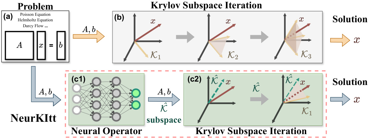
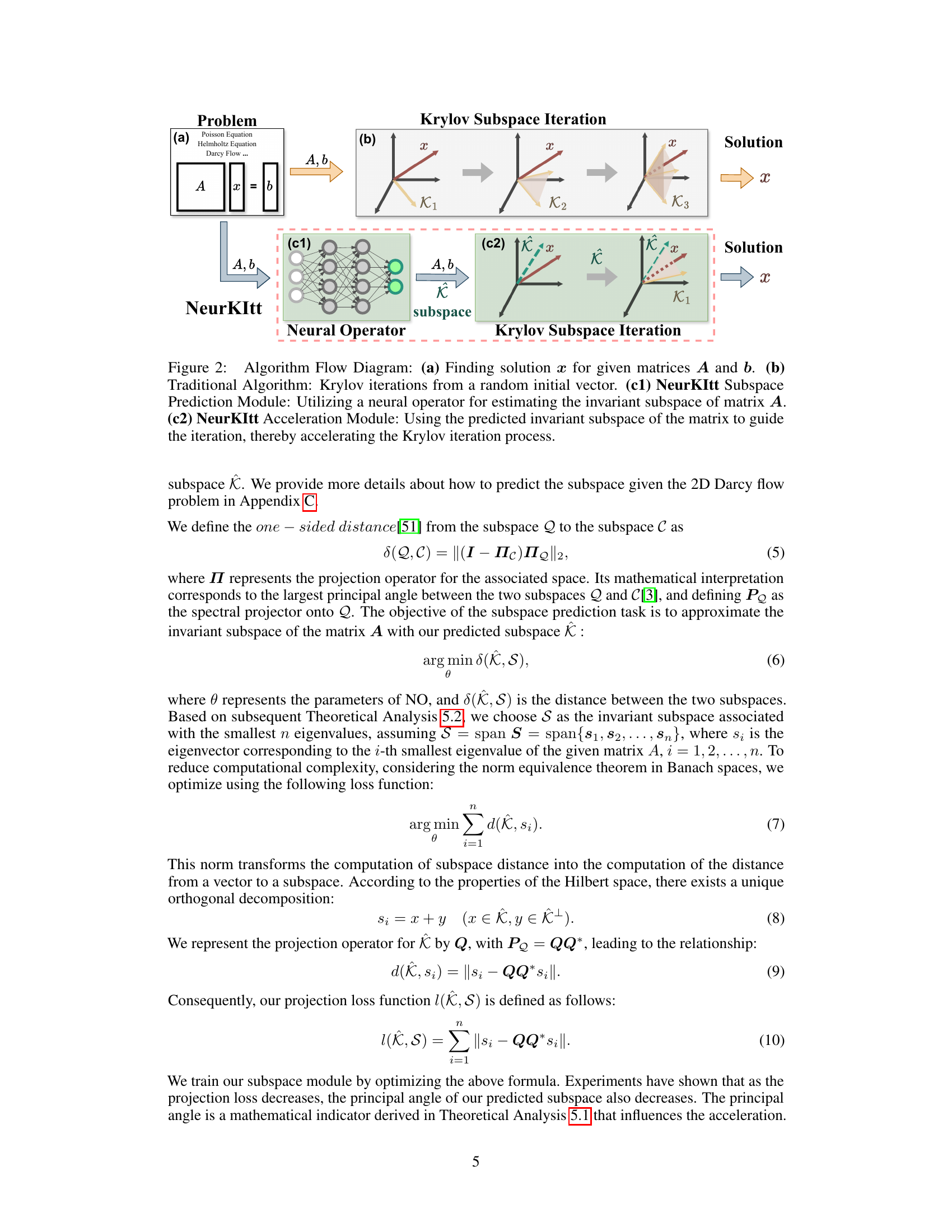
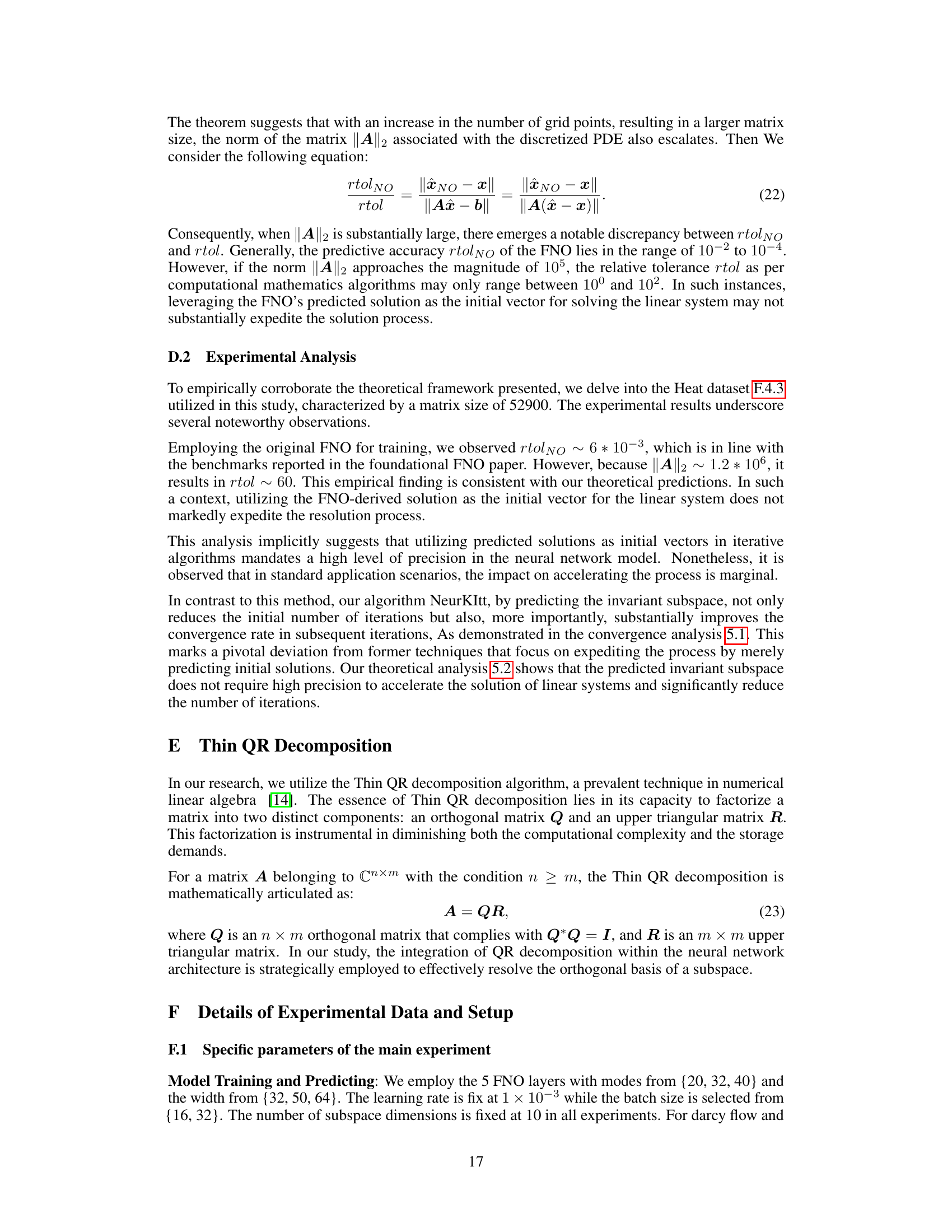
This figure illustrates the workflow of the proposed NeurKItt algorithm compared to traditional Krylov subspace iteration methods. Panel (a) shows the problem setup: finding the solution vector x for a given matrix A and vector b. Panel (b) illustrates the traditional Krylov subspace method, starting from a random initial vector and iteratively expanding the subspace to approximate the solution. Panel (c1) depicts the NeurKItt subspace prediction module, which uses a neural operator to predict the invariant subspace of the matrix A. Panel (c2) shows how the predicted subspace (from c1) is used to guide the Krylov subspace iteration in the acceleration module, resulting in a faster convergence to the solution.

This figure compares the performance of NeurKItt against GMRES for solving linear systems. It shows the convergence (tolerance) over time (left) and the average number of iterations (right) for both methods across various preconditioning techniques (Jacobi, BJacobi, SOR, ASM, ICC, ILU). NeurKItt demonstrates significantly faster convergence, requiring fewer iterations and less time to achieve the same tolerance.
This figure compares the performance of NeurKItt and GMRES in solving linear systems. The y-axis shows the 2-norm of the residual error (tolerance), and the x-axis shows either the computation time in seconds (left) or the number of iterations (right). Multiple lines represent different preconditioning techniques used with each solver. The results demonstrate that NeurKItt significantly reduces both the time and the number of iterations required to achieve a given level of accuracy, showing improvements of up to 5.5x and 16.1x respectively.

This figure compares the performance of the proposed Neural Krylov Iteration (NeurKItt) method against the Generalized Minimal Residual (GMRES) method for solving linear systems. It shows how the tolerance (2-norm) decreases over time (in seconds) and the number of iterations for various preconditioning techniques (None, Jacobi, BJacobi, SOR, ASM, ICC, ILU). The results demonstrate that NeurKItt significantly outperforms GMRES in both speed and iteration count, achieving up to a 5.5x speedup in time and a 16.1x speedup in iterations.
More on tables
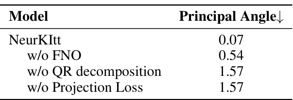
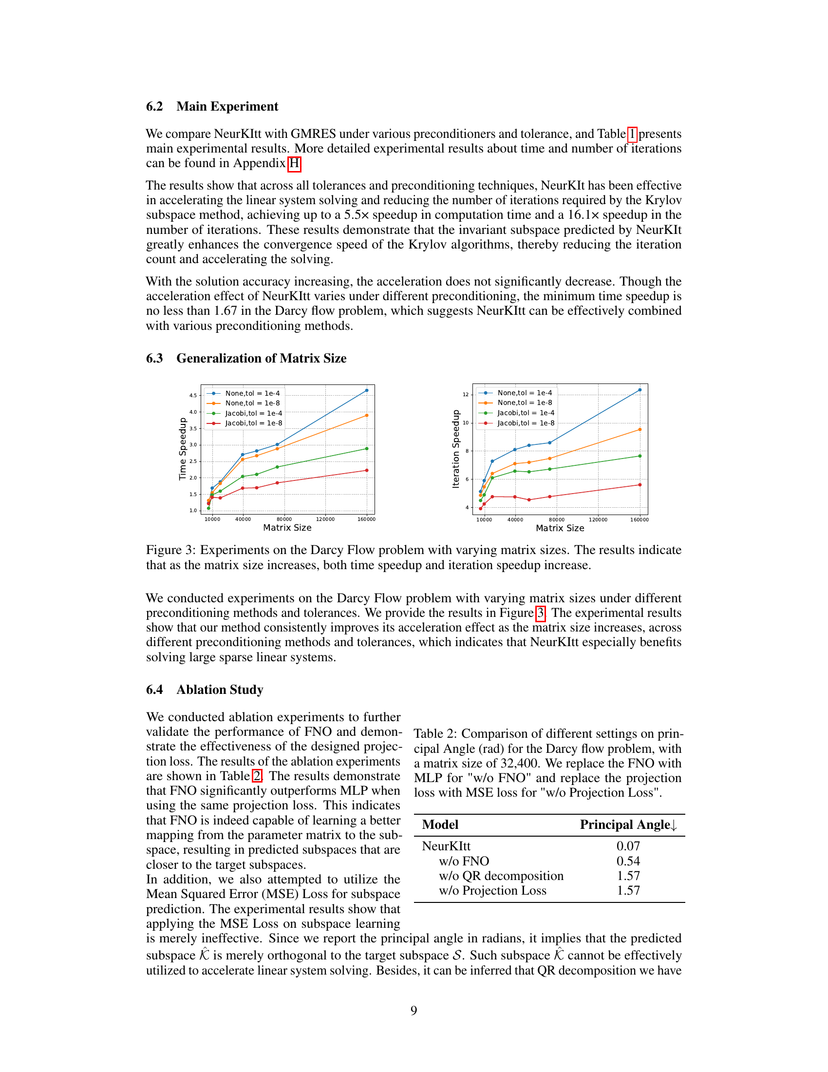
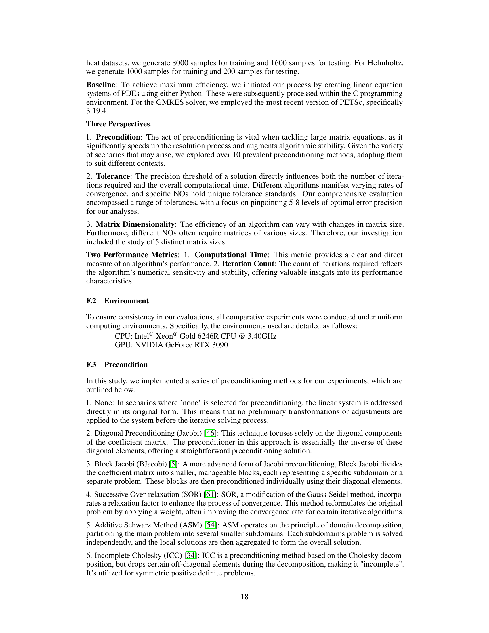
This table presents the ablation study results for the Darcy flow problem with a matrix size of 32,400. It compares the principal angle (a measure of subspace similarity) obtained using the full NeurKItt model against variations where either the Fourier Neural Operator (FNO), QR decomposition, or projection loss are removed. The principal angle is a measure of the difference between the predicted subspace and the actual invariant subspace; smaller angles indicate better predictions. The results show that FNO and the projection loss are crucial for accurate subspace prediction.

This table compares the performance of NeurKItt and GMRES in solving linear systems. It shows the speedup (both in computation time and number of iterations) achieved by NeurKItt compared to GMRES across various datasets (Darcy, Heat, Helmholtz), preconditioning techniques (None, Jacobi, BJacobi, SOR, ASM, ICC, ILU), and tolerance levels (1e-2, 1e-4, 1e-7, 1e-10, 1e-12). A speedup greater than 1 indicates that NeurKItt outperforms GMRES.

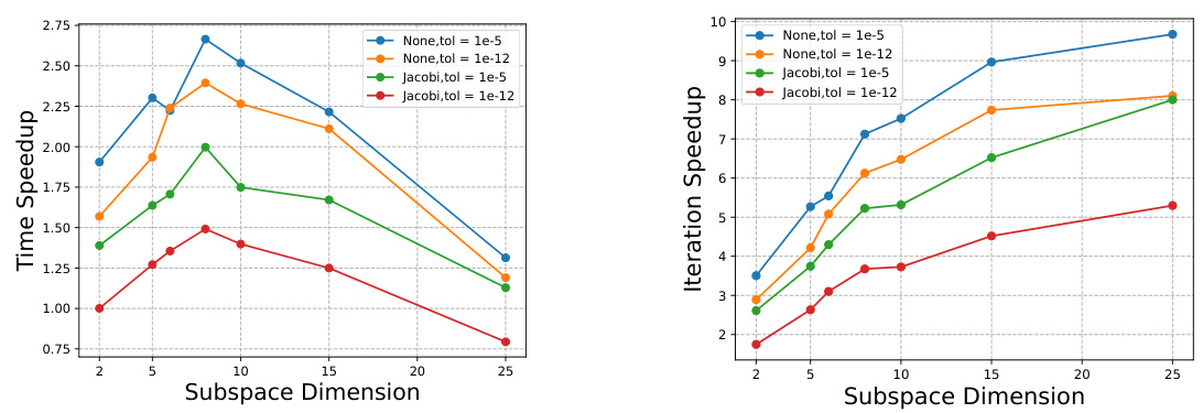
This table presents the results of experiments conducted to evaluate the impact of changing the number of layers, modes, and width in the Fourier Neural Operator (FNO) component of NeurKItt. The Darcy Flow problem was used with a fixed matrix size of 32400, a tolerance of 1e-5, and no preconditioning. The subspace dimension was held constant at 20. The table shows the principal angle (a measure of how well the predicted subspace aligns with the true invariant subspace), the time speedup (the ratio of GMRES solving time to NeurKItt solving time), and the iteration speedup (the ratio of GMRES iterations to NeurKItt iterations) for different layer, mode, and width configurations.

This table shows the inference time in milliseconds for the subspace prediction module. The inference time is quite low across all three datasets (Helmholtz, Heat, and Darcy), ranging from approximately 6 to 8 milliseconds. This demonstrates the efficiency of the subspace prediction module, as this computation time is negligible compared to the overall solving time of the linear system.

This table presents the training time in hours for the subspace prediction module of the NeurKItt algorithm. The training was conducted for 120 epochs on three different datasets: Helmholtz (62500), Heat (90000), and Darcy (160000). The table shows that the training time varies significantly across datasets, likely due to differences in dataset size and complexity. The Helmholtz dataset required significantly less training time (0.51 hours) compared to the Heat (6.48 hours) and Darcy (10.47 hours) datasets.

This table compares the performance of NeurKItt and GMRES across various datasets, preconditioning techniques, and tolerance levels. For each combination, it shows the speedup achieved by NeurKItt in terms of both computation time and the number of iterations required, relative to GMRES. The speedup values represent the ratio of GMRES time/iterations to NeurKItt time/iterations. A value greater than 1 indicates that NeurKItt is faster or uses fewer iterations.

This table presents a comparison of the performance of NeurKItt and GMRES across various datasets, preconditioning techniques, and tolerance levels. The ’time speedup’ represents the ratio of GMRES solving time to NeurKItt solving time, indicating how much faster NeurKItt is. Similarly, ‘iteration speedup’ shows the ratio of the number of iterations used by GMRES to the number used by NeurKItt. The data demonstrates NeurKItt’s acceleration capabilities under different conditions.
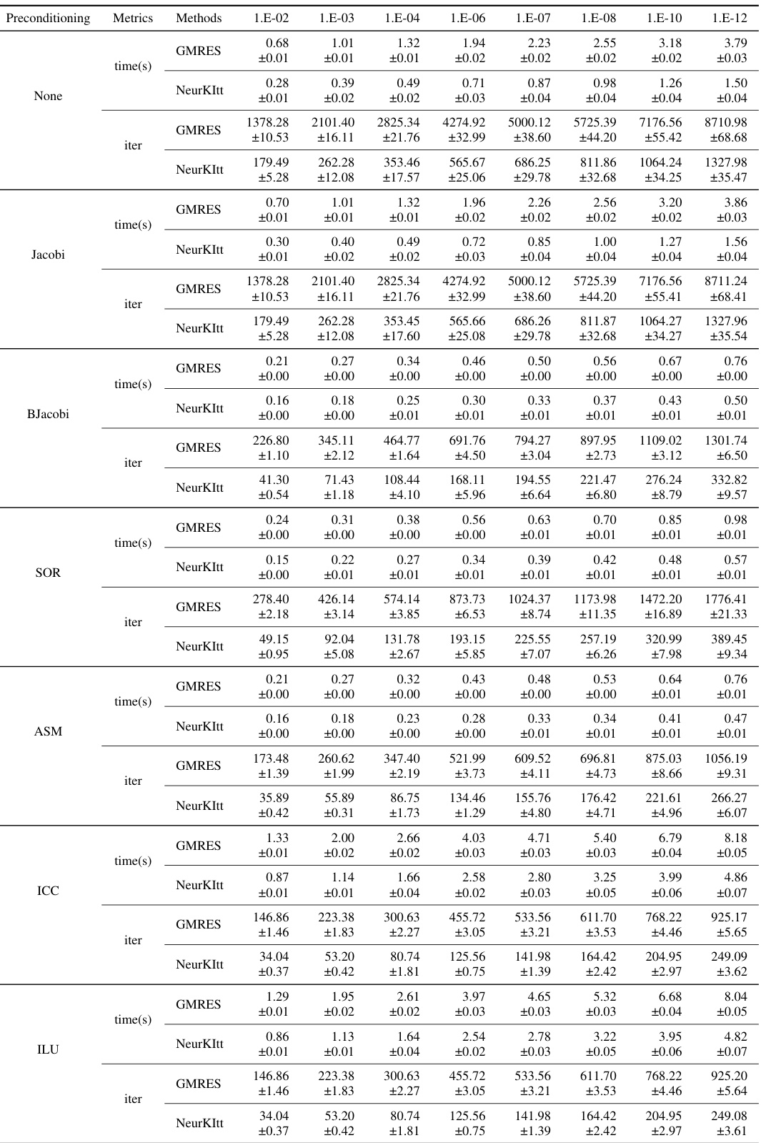
This table presents a comparison of the performance of NeurKItt and GMRES, two algorithms used for solving linear systems. The comparison is done across various datasets (Darcy, Heat, Helmholtz), preconditioning techniques (None, Jacobi, BJacobi, SOR, ASM, ICC, ILU), and tolerances (1e-2, 1e-4, 1e-7, 1e-10, 1e-12). The results are expressed as the speedup factor achieved by NeurKItt relative to GMRES in both computation time and number of iterations.

This table compares the performance of NeurKItt and GMRES in solving linear systems. It shows the time speedup and iteration speedup achieved by NeurKItt relative to GMRES across various datasets (Darcy, Heat, Helmholtz), preconditioning techniques (None, Jacobi, BJacobi, SOR, ASM, ICC, ILU), and tolerance levels (1e-2, 1e-4, 1e-7, 1e-10, 1e-12). Higher values indicate better performance for NeurKItt.
Full paper#
