↗ OpenReview ↗ NeurIPS Proc. ↗ Chat
TL;DR#
Many recent studies have explored using large language models (LLMs) for time series forecasting, assuming that LLMs’ ability to handle sequential data in natural language will translate to improved performance in time series. However, this paper challenges that assumption. The authors conduct a series of ablation studies on three popular LLM-based forecasting methods, systematically removing or replacing the LLM component with simpler alternatives such as basic attention layers.
The results show that removing or replacing the LLM component does not negatively impact forecasting performance; in many cases, performance even improves! This suggests that the computational overhead associated with using LLMs in time series forecasting is not justified by any performance gains. The researchers further investigate the role of different time series encoders, finding that simple patching and attention mechanisms perform comparably to the more complex LLM-based approaches. This challenges the prevailing trend of incorporating LLMs into time-series modeling and suggests a more critical and selective approach is needed.
Key Takeaways#
Why does it matter?#
This paper is crucial because it challenges the prevailing assumption that large language models automatically improve time series forecasting. By systematically evaluating several popular LLM-based methods and their simpler alternatives, it reveals the unexpected finding that LLMs offer no significant advantages in forecasting accuracy and instead often increase computational costs. This has significant implications for resource allocation in time-series research, prompting a more critical approach to LLM adoption. The study also provides valuable insights into the components of time-series encoders, guiding future research towards more efficient and effective methods.
Visual Insights#

This figure illustrates the four different models used in the ablation study. (a) shows a standard LLM-based model for time series forecasting, where the LLM can be either frozen or fine-tuned. (b), (c), and (d) show ablation models where the LLM is removed, replaced with a self-attention layer, and replaced with a Transformer block, respectively. Each ablation isolates the effect of the LLM to understand its contribution to the forecasting performance.

This table presents the characteristics of eight datasets used in the paper to evaluate the performance of language models in time series forecasting. The datasets cover various domains such as energy, weather, traffic, and finance, and exhibit different characteristics in terms of the number of channels, sampling rates, and total timesteps.
In-depth insights#
LLM Forecasting Use#
The utility of large language models (LLMs) for time series forecasting is a subject of ongoing debate. This research investigates the actual contribution of LLMs in three prominent LLM-based forecasting methods. The core finding is that removing the LLM component or replacing it with simpler alternatives like a basic attention layer does not significantly reduce forecasting accuracy; in many cases, accuracy even improves. This suggests that the computational expense associated with pretrained LLMs offers minimal benefit over simpler, more efficient models. Further, the study demonstrates that LLMs do not inherently enhance the representation of sequential dependencies in time series, challenging the often-assumed synergy between language models and time series. Few-shot learning is also found not to be improved by LLMs, indicating their limitations in data-scarce scenarios. Overall, the research emphasizes the need for caution in applying computationally expensive LLMs to time series forecasting, suggesting a re-evaluation of current methodologies is warranted. Simpler models offer comparable or superior performance with substantially reduced computational requirements.
Ablation Study Design#
A well-designed ablation study systematically removes or alters components of a model to isolate their individual contributions. In the context of this research paper, an ablation study would likely involve removing the LLM component entirely from existing LLM-based time series forecasting models, replacing the LLM with simpler alternatives (e.g., basic attention mechanisms or transformer blocks), or varying the LLM’s training parameters to analyze their effect on performance. The primary goal is to determine whether the LLM is essential for successful forecasting or if its contribution is negligible or even detrimental compared to simpler and more computationally efficient approaches. A thorough ablation study should test these modifications across a range of datasets and prediction horizons, comparing the results to the original LLM-based methods. Careful consideration should be given to the selection of simpler models for substitution, ensuring they maintain relevant architectural features and possess similar complexity. The results could reveal whether the LLM’s inherent architecture offers any advantage in the time-series forecasting context, providing valuable insights into its true value and potential areas for improvement or replacement. A focus on both performance metrics (such as MAE and MSE) and computational efficiency is crucial to fully assess the impact of the different model components.
Time Series Encoders#
The effectiveness of various time series encoders is a crucial aspect of this research. The study directly compares the performance of LLM-based encoders against simpler alternatives like patching and attention mechanisms. This comparison is essential because LLM-based methods, while conceptually appealing, are computationally expensive. The findings reveal that simpler encoders perform comparably, if not better, than the LLM-based ones, highlighting the potential inefficiency of leveraging LLMs for this specific task. This challenges the common assumption that the advanced sequential modeling capabilities of LLMs inherently translate to superior performance in time series forecasting. Further investigation into the reasons for this unexpected result is needed, focusing on the limitations of transferring knowledge learned from text data to time series data, as well as the potential redundancy of complex LLM architectures when basic attention structures prove equally effective.
Computational Costs#
The research paper highlights the significant computational costs associated with using large language models (LLMs) in time series forecasting. While LLMs offer the potential for advanced sequence modeling, the study demonstrates that simpler methods achieve comparable or even superior performance with substantially less computational overhead. This discrepancy is a crucial finding, suggesting that the benefits of LLMs in this context may not outweigh their high resource demands. The orders-of-magnitude difference in training and inference time between LLM-based approaches and their ablations underscores the need for careful consideration of computational efficiency when choosing forecasting methods. Pretrained LLMs were shown to offer no advantage over models trained from scratch, further diminishing their value given their considerable computational expense. Therefore, prioritizing computationally efficient alternatives should be a primary concern in time series forecasting applications, especially when dealing with large or complex datasets.
Future Research#
Future research could explore several promising avenues. Extending the ablation studies to a wider range of LLMs and time series datasets is crucial to validate the findings more broadly. Investigating the potential benefits of LLMs in multimodal time series analysis, where textual data complements numerical time series, is another important direction. Developing novel architectures that specifically leverage the strengths of LLMs for time-series reasoning, perhaps through symbolic reasoning or hybrid models, could unlock significant improvements in forecasting accuracy. Finally, exploring the use of LLMs for tasks such as anomaly detection, classification, and imputation, beyond traditional forecasting, warrants further investigation. A deeper understanding of how LLMs interact with various time series encoding techniques could lead to improved model designs. Focus should be placed on efficient and computationally tractable methods that avoid the high cost associated with current LLM-based models.
More visual insights#
More on figures

This figure illustrates four different models for time series forecasting. Model (a) uses a pre-trained large language model (LLM) as the core component. In models (b), (c), and (d), the LLM is ablated: (b) the LLM is entirely removed; (c) the LLM is replaced with a single self-attention layer; (d) the LLM is replaced with a simple Transformer block. This allows the authors to isolate the impact of the LLM on forecasting performance.

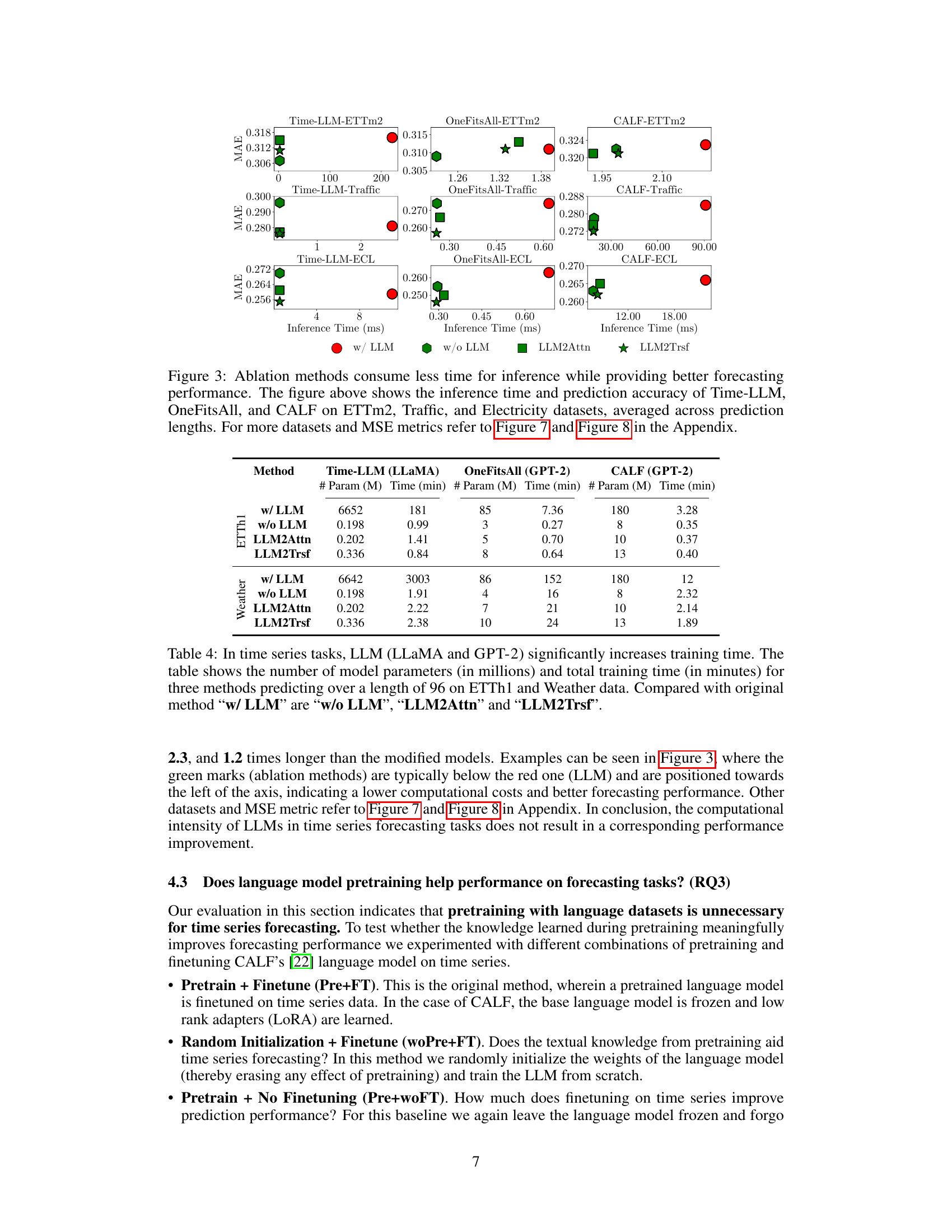
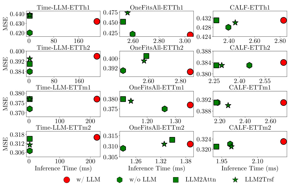
This figure compares the inference time and prediction accuracy (MAE) of three popular LLM-based time series forecasting methods (Time-LLM, OneFitsAll, and CALF) against their ablated versions (w/o LLM, LLM2Attn, LLM2Trsf) across three different datasets (ETTm2, Traffic, and Electricity). The results are averaged across various prediction lengths. The key takeaway is that the ablation methods generally achieve comparable or better forecasting accuracy while significantly reducing inference time, suggesting the LLM component is not essential for good performance.

This figure illustrates the four different methods used for time series forecasting in the paper. (a) shows the standard method of using an LLM. (b) shows a model without the LLM, (c) shows one using a self-attention layer instead of the LLM and (d) one with a Transformer instead of the LLM.
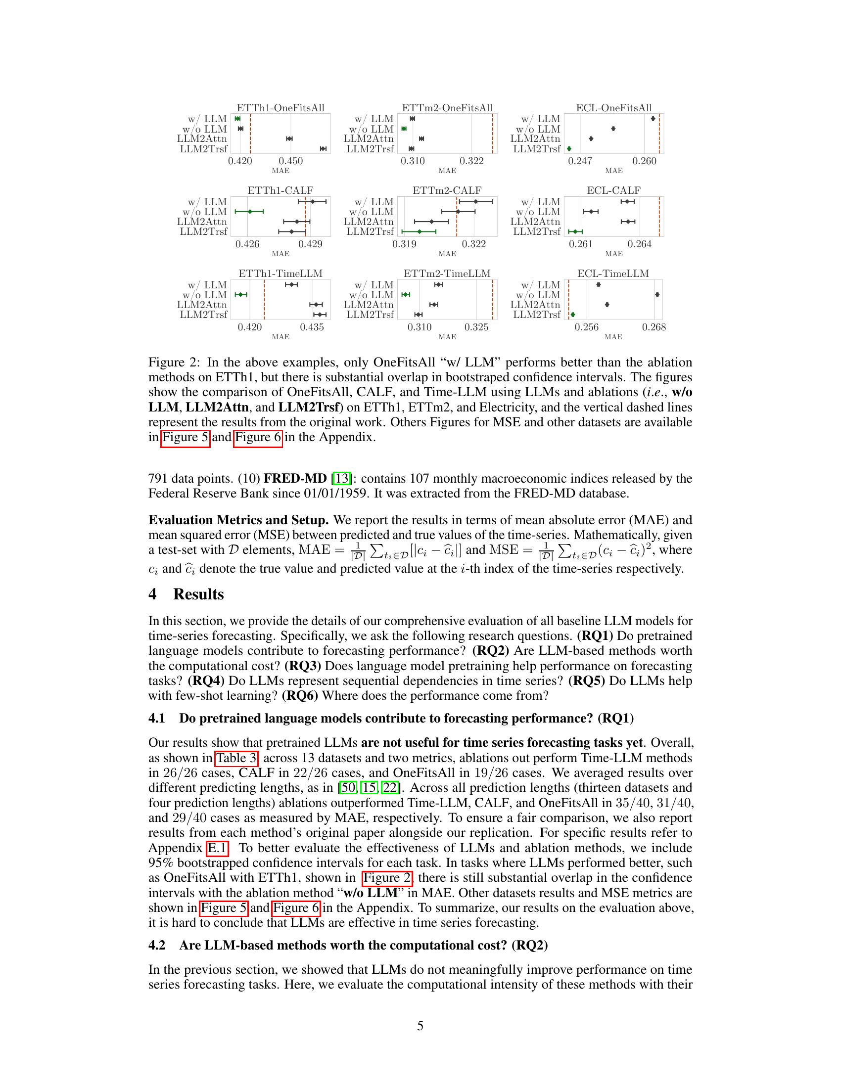
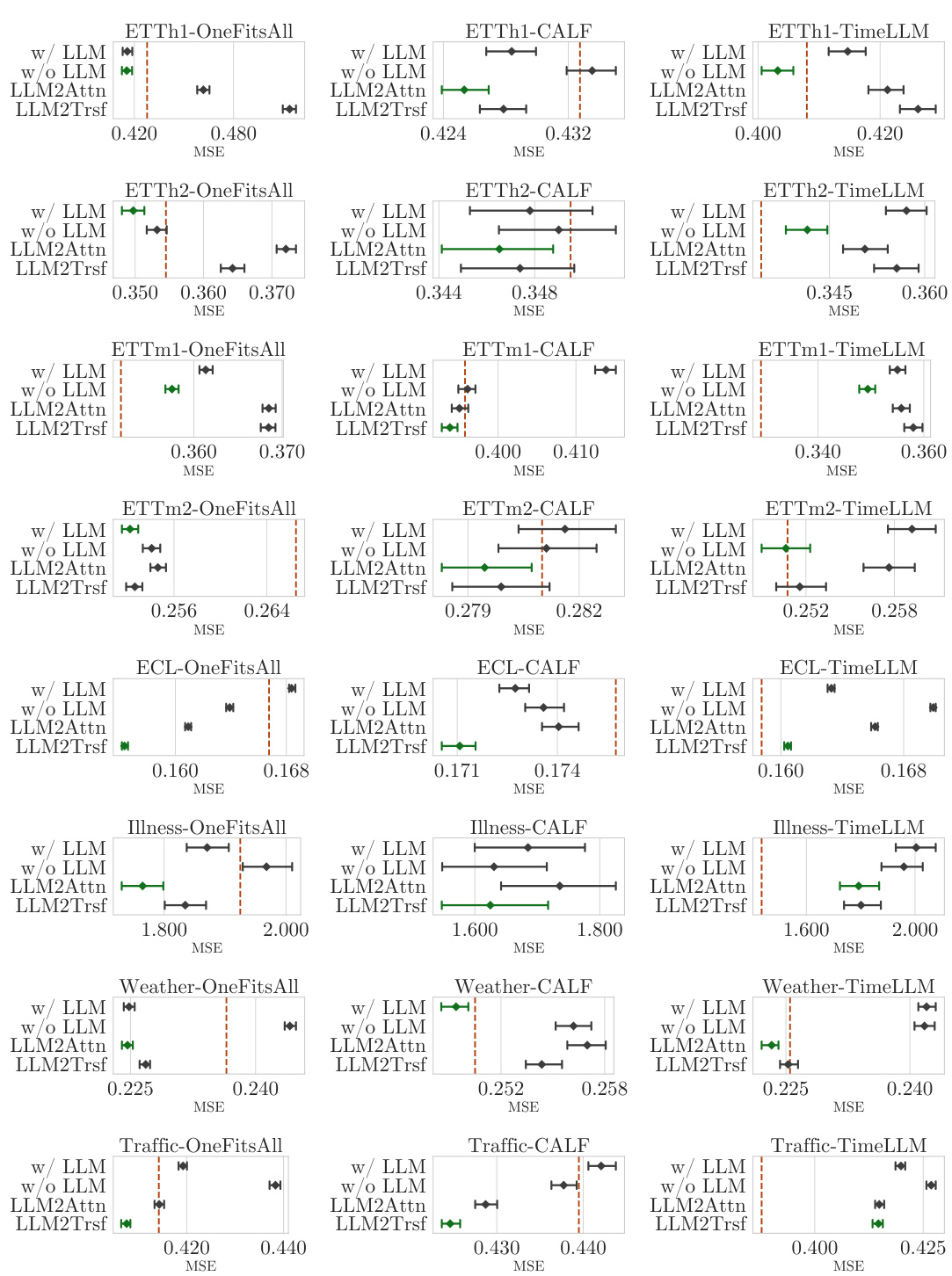
The figure compares the performance of three popular LLM-based time series forecasting methods (OneFitsAll, CALF, and Time-LLM) against their ablations (removing the LLM component or replacing it with simpler structures). The results show that in most cases, simpler methods perform comparably or even better than the original LLM-based methods, especially considering the substantial reduction in computational cost. The figure showcases this performance comparison across three different datasets (ETTh1, ETTm2, and Electricity) and using the MAE metric. Bootstrapped confidence intervals are used to account for variability in the results.
This figure illustrates the four different ablation methods used in the paper to evaluate the impact of LLMs in time series forecasting. The first setup uses a pretrained LLM, while the others progressively remove or replace parts of the LLM with simpler components to analyze the contribution of the LLM to the overall performance. Each panel shows a simplified diagram of the model architecture.

This figure illustrates the four different models used in the ablation study. The first model uses a pre-trained Large Language Model (LLM) as the core of the time series forecasting model, showing both frozen and fine-tuned variations. The next three models demonstrate the ablations: removing the LLM entirely, replacing it with a self-attention layer, and replacing it with a Transformer block. Each ablation modifies the original LLM-based model to isolate the impact of the LLM on forecasting performance.
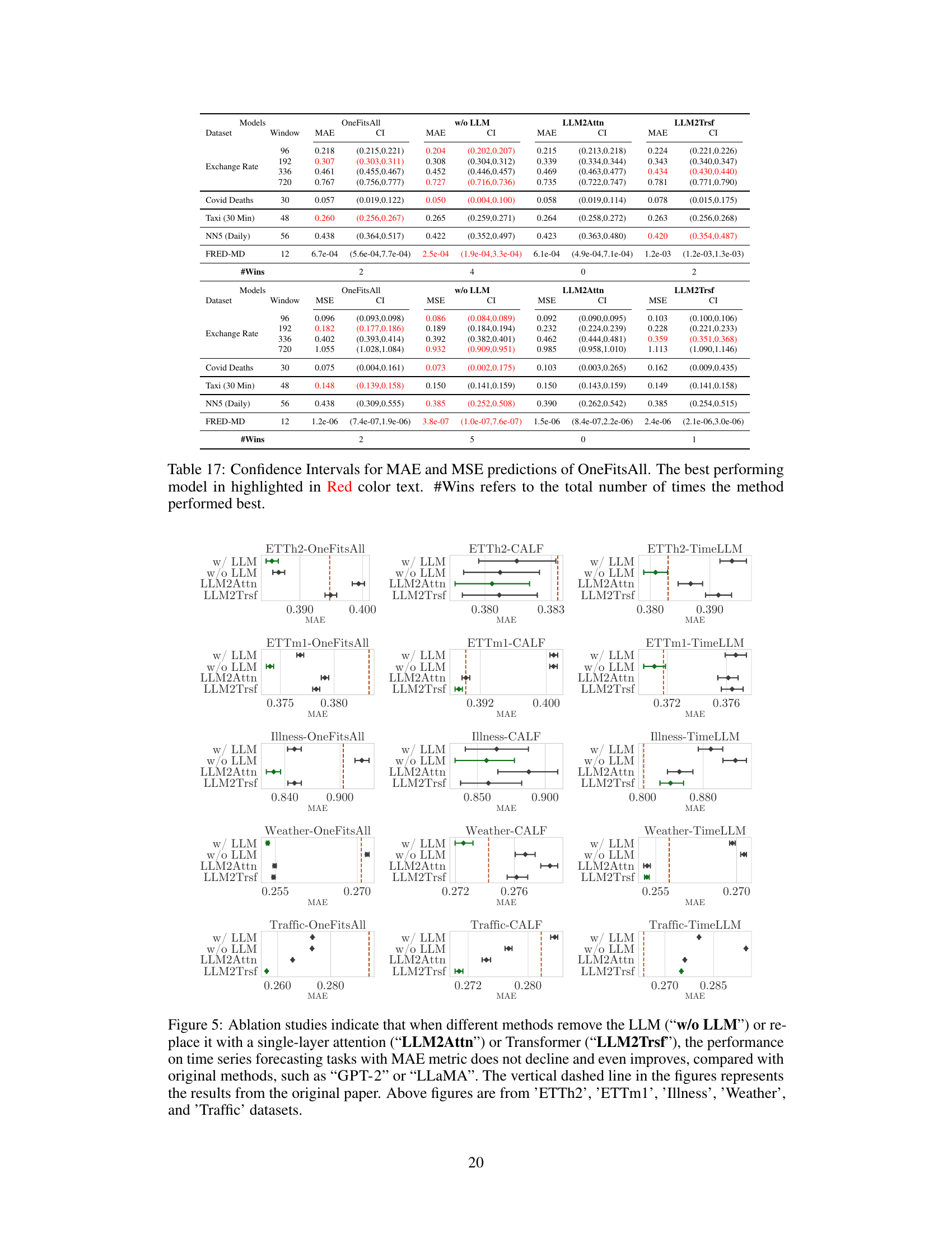
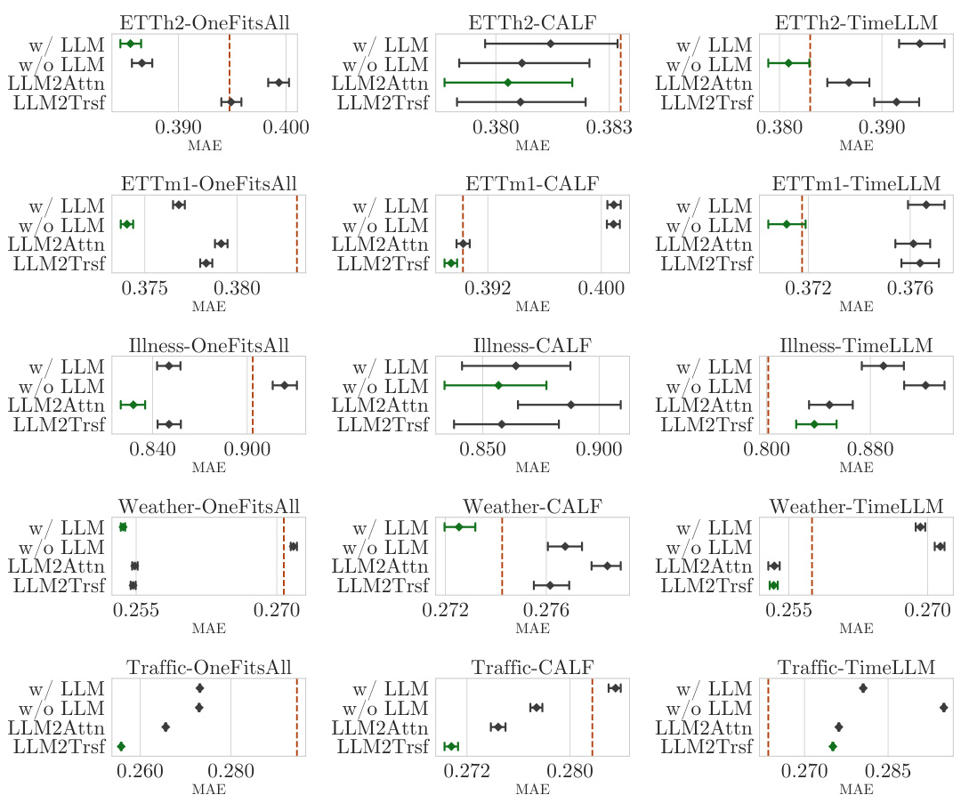
This figure shows the results of ablation studies on three popular LLM-based time series forecasting methods. It demonstrates that removing the LLM component or replacing it with simpler architectures (a single-layer attention or a transformer block) does not negatively impact forecasting performance, and in many cases, even improves it. The results are shown using the MAE (Mean Absolute Error) metric across several datasets, comparing the original LLM-based models with their ablated versions. The vertical dashed lines represent the results reported in the original papers for comparison.
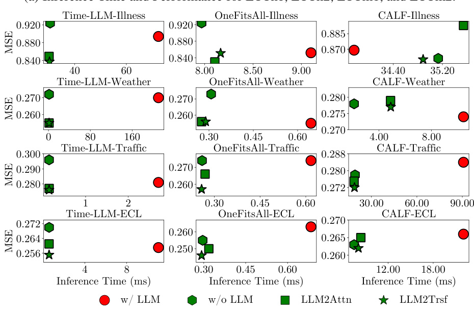
The figure shows that using LLMs for time series forecasting increases inference time by orders of magnitude, while not improving forecasting accuracy. Ablation studies, which remove or replace the LLM component with simpler models, show comparable or better performance with significantly reduced inference time. This suggests that the computational overhead of LLMs does not translate to better forecasting accuracy in the context of time series analysis.
More on tables

This table summarizes three popular methods for time series forecasting that utilize large language models (LLMs). It shows the base model used (GPT-2 or LLaMA), how the LLM parameters are handled (learnable or frozen), whether positional and word embeddings are used, and if the method is multimodal.
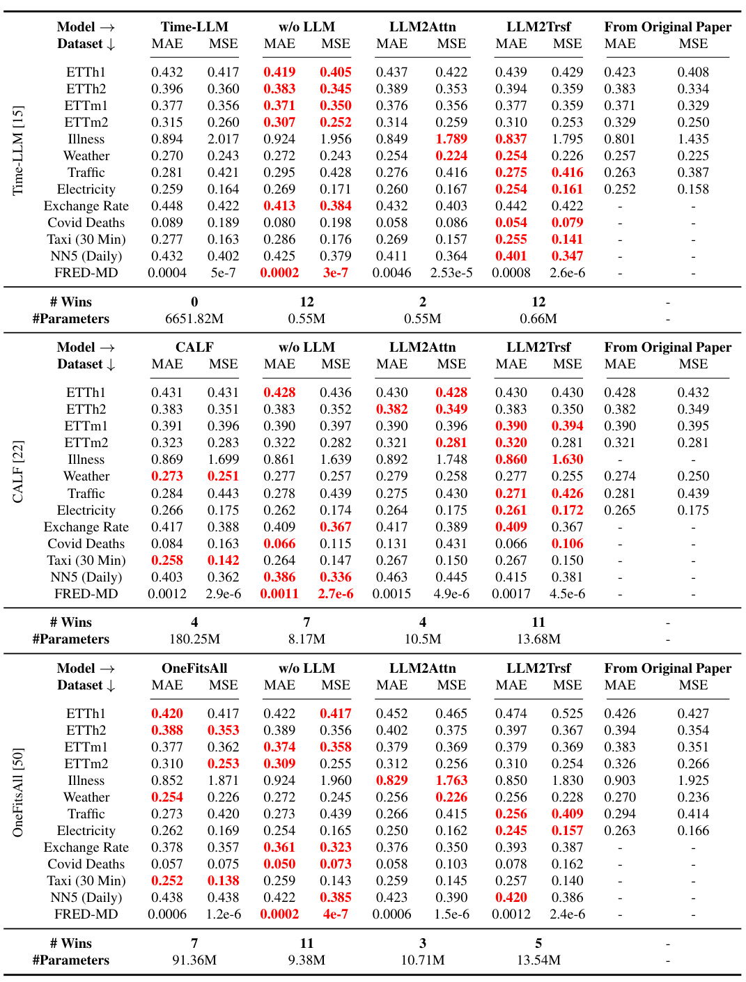
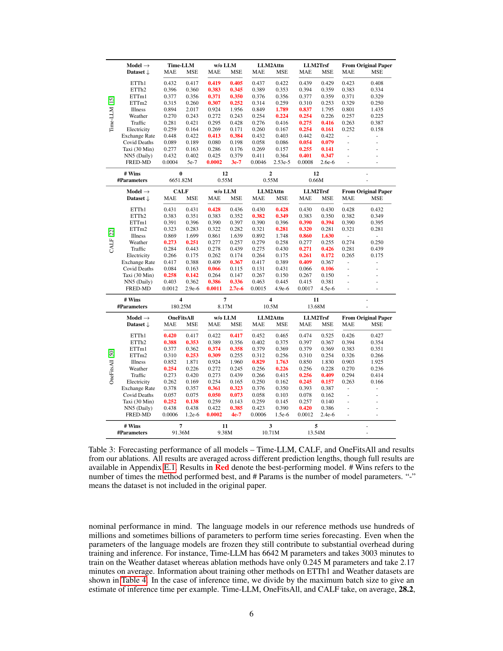
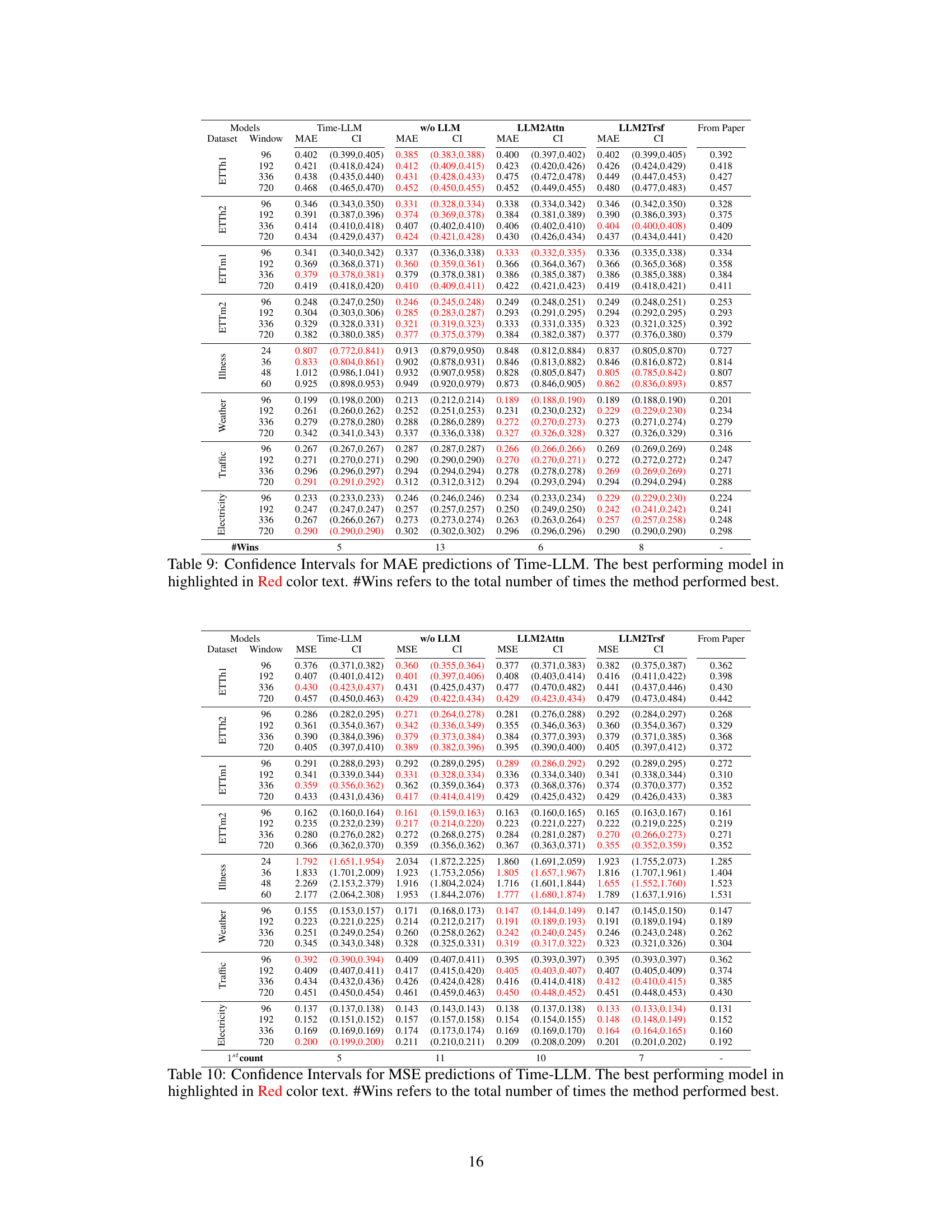
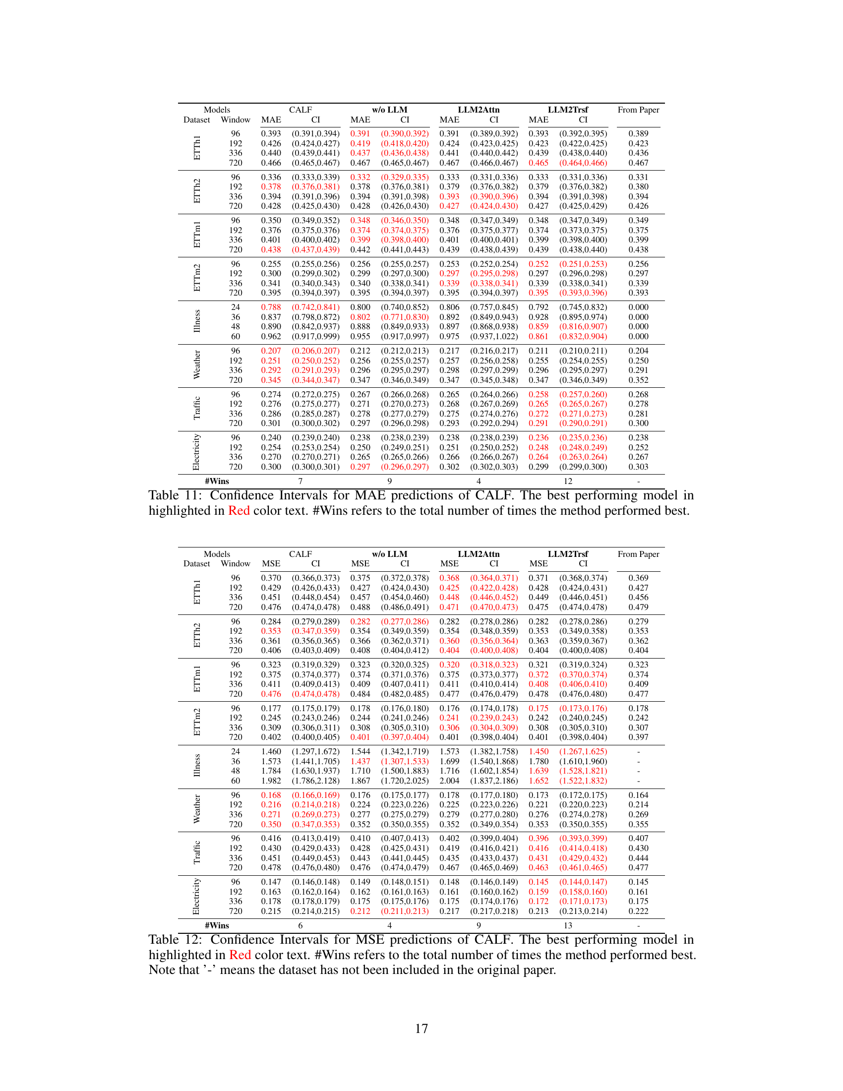
This table presents the forecasting performance results for three popular LLM-based time series forecasting methods (Time-LLM, CALF, OneFitsAll) and their corresponding ablation models (w/o LLM, LLM2Attn, LLM2Trsf). The results are averaged over different prediction lengths, with the best-performing model highlighted in red. The table also provides the number of times each model achieved the best performance (# Wins) and the number of model parameters (# Params). Datasets not included in the original papers are indicated with a ‘-’.
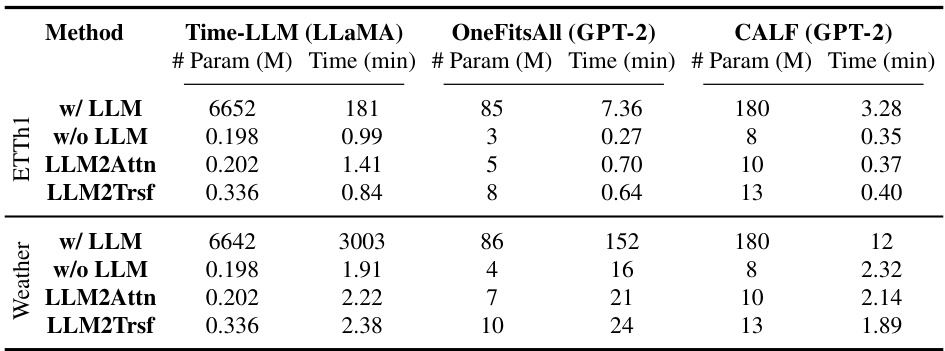
This table compares the computational cost (in terms of model parameters and training time) of three different methods for time series forecasting: Time-LLM, OneFitsAll, and CALF. For each method, it shows the resources required when using the full language model (‘w/ LLM’) and after applying three ablations: removing the LLM (‘w/o LLM’), replacing the LLM with an attention layer (‘LLM2Attn’), and replacing the LLM with a transformer block (‘LLM2Trsf’). The table highlights the significant increase in computational cost associated with using the full LLMs for time series forecasting tasks.
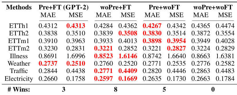
This table presents the results of an ablation study comparing four different training approaches for LLMs in time series forecasting. The methods compared are: Pretraining + Finetuning (Pre+FT), Random Initialization + Finetuning (woPre+FT), Pretraining + No Finetuning (Pre+woFT), and Random Initialization + No Finetuning (woPre+woFT). The table shows the MAE and MSE for each method across eight different datasets. The results demonstrate that randomly initializing the LLM parameters and training from scratch generally outperforms using a pretrained model, regardless of whether fine-tuning is used.
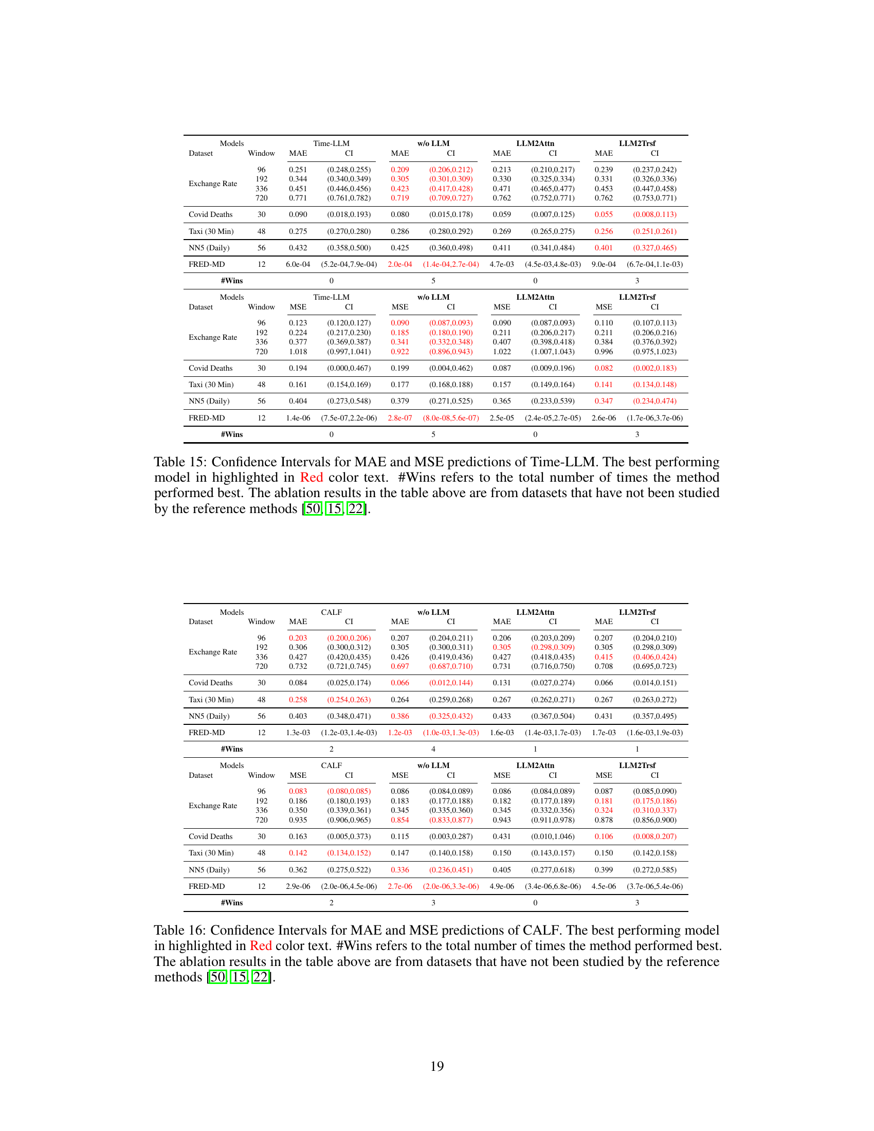
This table presents a comparison of the forecasting performance (MAE and MSE) of three popular LLM-based time series forecasting methods (Time-LLM, CALF, OneFitsAll) and their corresponding ablations (without LLM, LLM replaced with attention, LLM replaced with transformer). The results are averaged across various prediction lengths and presented for thirteen datasets. The table highlights the best-performing model for each dataset and metric and shows the number of times each model achieved the best performance (# Wins) and the number of parameters (#Params) for each model.

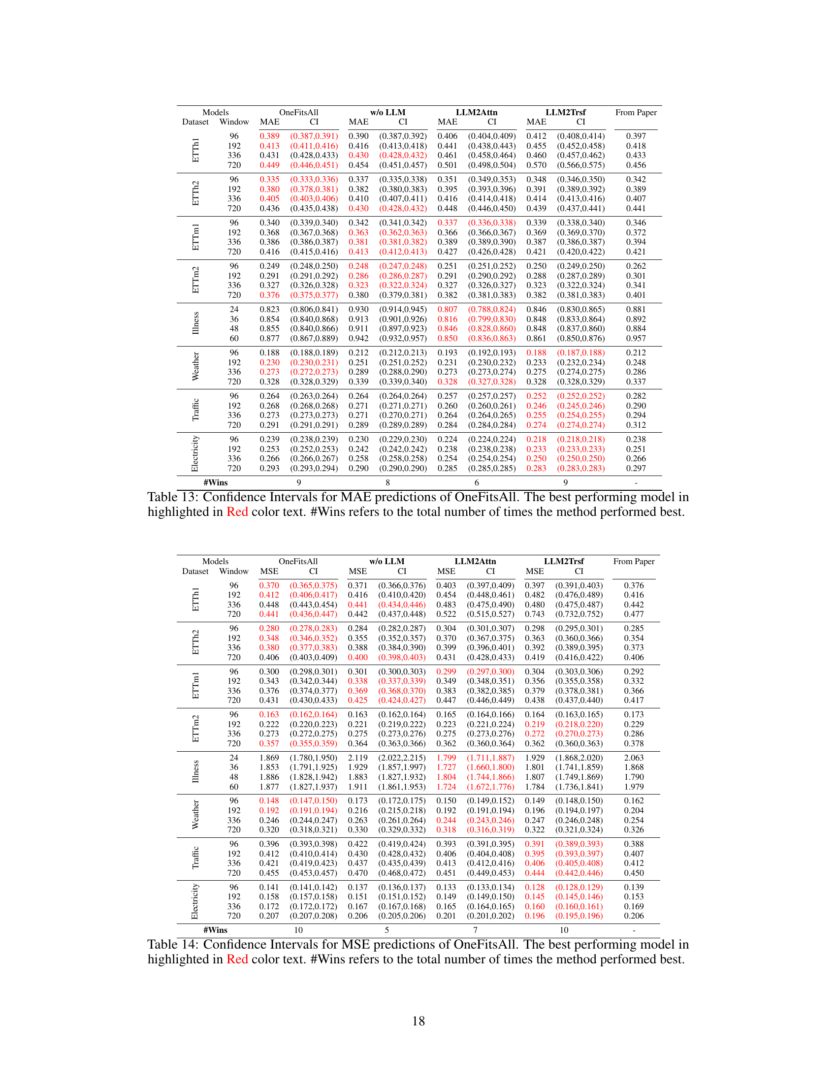
This table presents the forecasting performance (MAE and MSE) of three popular LLM-based time series forecasting methods (Time-LLM, CALF, OneFitsAll) and their corresponding ablation methods (w/o LLM, LLM2Attn, LLM2Trsf). The results are averaged across various prediction lengths for better evaluation. The table highlights the best-performing model for each dataset and metric, providing a clear comparison of the performance gain or loss due to the LLM component. Additionally, it shows the number of times each method achieved the best performance and the number of parameters used in each model.

This table presents a comparison of the forecasting performance (MAE and MSE) of three popular LLM-based time series forecasting methods (Time-LLM, CALF, OneFitsAll) and their corresponding ablation versions (without LLM, LLM replaced with attention, LLM replaced with transformer). The results are averaged across various prediction lengths and shown for multiple benchmark datasets. The table highlights the best-performing model for each dataset and metric, and counts the number of times each model achieves the best performance (Wins). It also provides the number of parameters for each model.

This table presents the forecasting performance results for three popular LLM-based time series forecasting methods (Time-LLM, CALF, OneFitsAll) and their corresponding ablation methods. The performance is measured using MAE and MSE metrics, averaged across multiple prediction lengths. The table also indicates the number of times each method achieved the best performance (’# Wins’) and the number of model parameters (’# Parameters’). The ‘-’ symbol signifies that a specific dataset was not used in the original paper’s experiments.
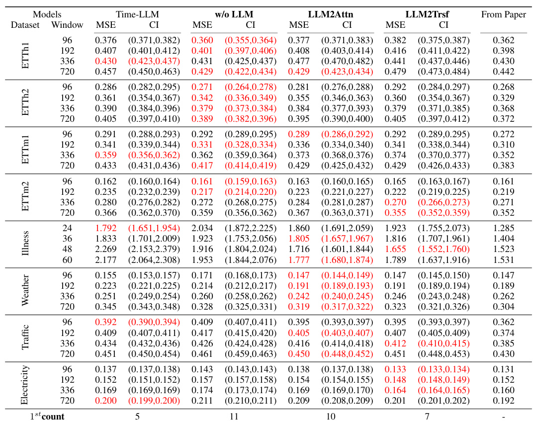
This table presents the forecasting performance of three popular LLM-based time series forecasting methods (Time-LLM, CALF, OneFitsAll) and their corresponding ablation studies (removing the LLM component, replacing it with a basic attention layer, or a basic transformer block). The performance is evaluated using MAE and MSE metrics across multiple datasets and prediction lengths. The table highlights the best-performing model for each scenario and indicates the number of times each method achieved the best performance. The number of model parameters is also shown for each model.
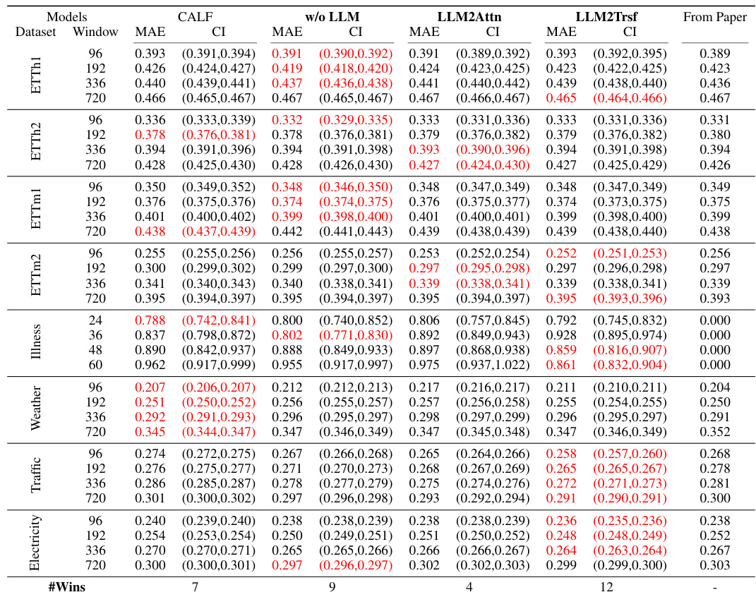
This table presents the forecasting performance results (MAE and MSE) for Time-LLM, CALF, and OneFitsAll models, along with their ablation variants. Results are averaged across different prediction lengths, providing a comprehensive comparison. The table highlights the best-performing models for each dataset and metric, indicating the number of times each method achieved the best performance. Note that some datasets are missing from certain methods’ original papers, represented by hyphens.
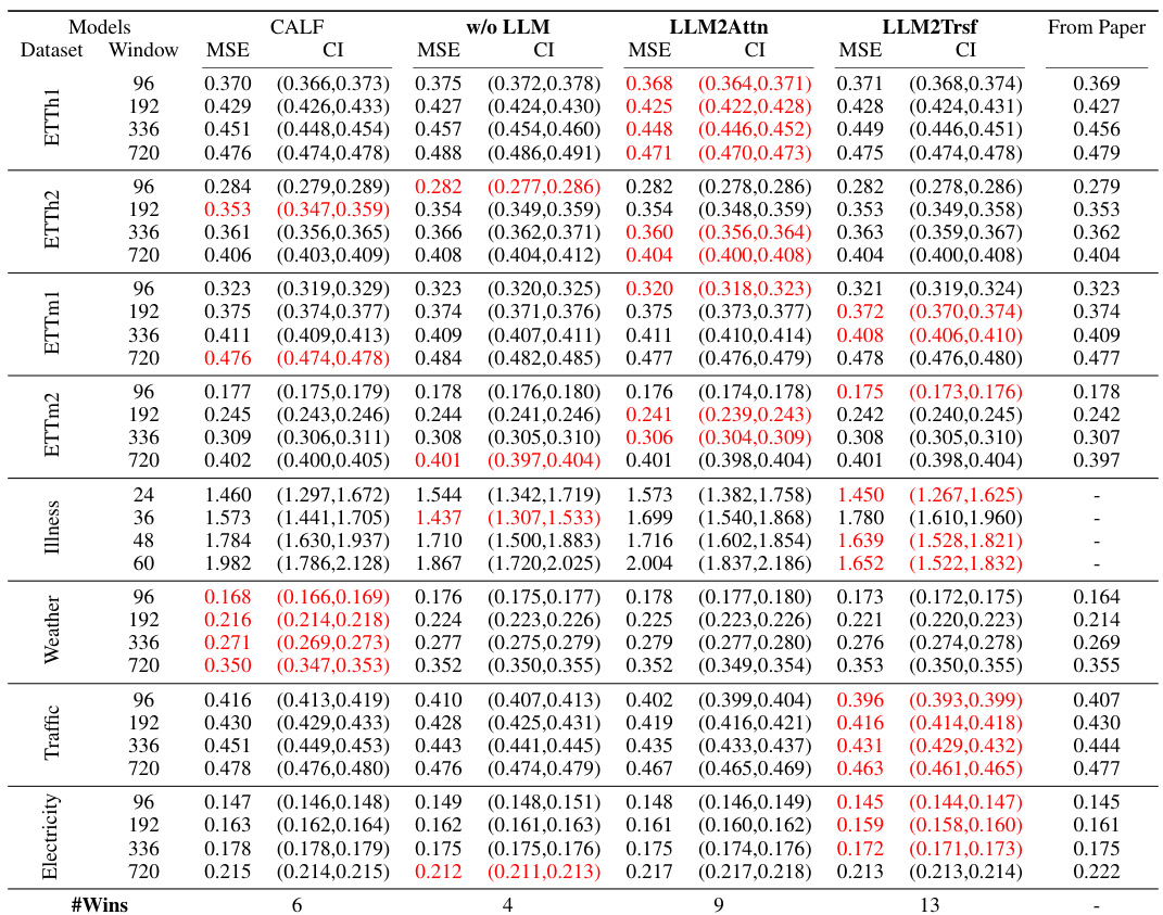
This table presents the forecasting performance results of three popular LLM-based time series forecasting methods (Time-LLM, CALF, OneFitsAll) and their corresponding ablation models (w/o LLM, LLM2Attn, LLM2Trsf). The performance is evaluated using MAE and MSE metrics across thirteen datasets and four prediction lengths. Results are color-coded to highlight the best-performing model for each scenario, and the number of times each model achieved the best performance is also provided. The table includes the number of parameters used by each model.
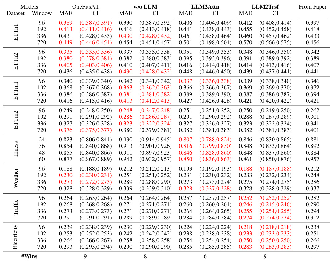
This table presents the forecasting performance results of three popular LLM-based time series forecasting methods (Time-LLM, CALF, and OneFitsAll) and their corresponding ablations (w/o LLM, LLM2Attn, and LLM2Trsf) across thirteen datasets. The performance is evaluated using MAE and MSE metrics averaged over different prediction lengths. The table also indicates which method achieved the best performance (# Wins) for each dataset and provides the number of parameters for each model. Results highlighted in red indicate the best-performing model for each metric and dataset combination.
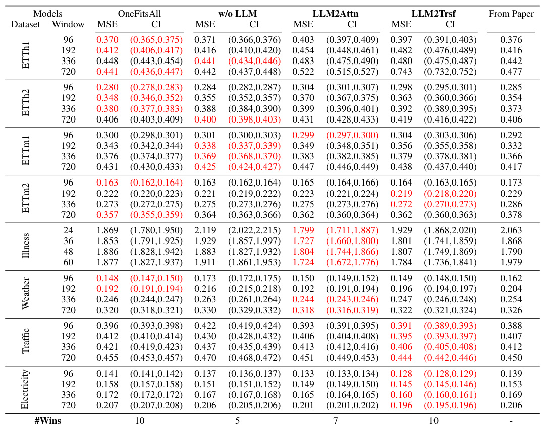
This table presents a comparison of the forecasting performance (MAE and MSE) of three popular LLM-based time series forecasting methods (Time-LLM, CALF, OneFitsAll) and their corresponding ablations (w/o LLM, LLM2Attn, LLM2Trsf) across thirteen datasets. The results are averaged across different prediction lengths. The table highlights the best performing model for each dataset and metric and provides the number of times each model achieved the best performance (#Wins) and the number of model parameters.
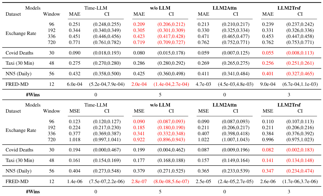
This table presents the forecasting performance results for three popular LLM-based time series forecasting methods (Time-LLM, CALF, OneFitsAll) and their corresponding ablation models (w/o LLM, LLM2Attn, LLM2Trsf). The results are averaged across various prediction lengths, with detailed results provided in Appendix E.1. The table highlights the best-performing model for each dataset and metric using red font, and indicates the number of times each model achieved the best performance (’# Wins’). It also indicates the number of parameters for each model.

This table presents the forecasting performance of three popular LLM-based time series forecasting methods (Time-LLM, CALF, OneFitsAll) and their corresponding ablation models (without LLM, LLM replaced with attention, LLM replaced with transformer). The performance is evaluated across 13 datasets using Mean Absolute Error (MAE) and Mean Squared Error (MSE) metrics, averaged across different prediction horizons. The table highlights the best-performing model for each dataset and metric and indicates the number of times each model achieved the best performance. It also shows the number of parameters for each model and indicates where datasets were not present in the original papers.
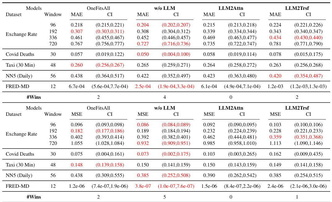
This table presents the forecasting performance results for three state-of-the-art LLM-based time series forecasting methods (Time-LLM, CALF, and OneFitsAll) and their corresponding ablation models. The results are averaged over different prediction horizons and presented for multiple benchmark datasets. The table highlights the best-performing model for each dataset/metric combination and shows the number of times each method achieved the best performance (‘Wins’) and the number of parameters for each model. Note that some datasets are not included in the original papers’ results.
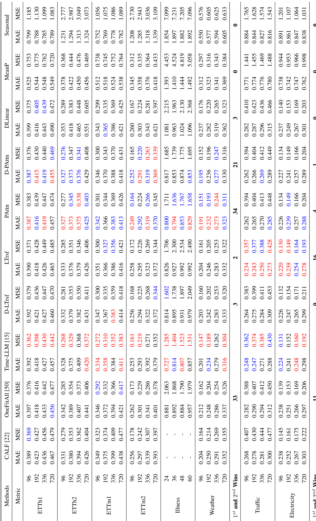
This table presents the forecasting performance results for three popular LLM-based time series forecasting methods (Time-LLM, CALF, OneFitsAll) and their corresponding ablation models (w/o LLM, LLM2Attn, LLM2Trsf). The results are averaged across different prediction lengths and presented for multiple datasets and metrics (MAE and MSE). The best performing model in each case is highlighted in red. The ‘# Wins’ column shows the number of times each model achieved the best performance across all datasets and prediction lengths, while ‘# Parameters’ indicates the number of model parameters.
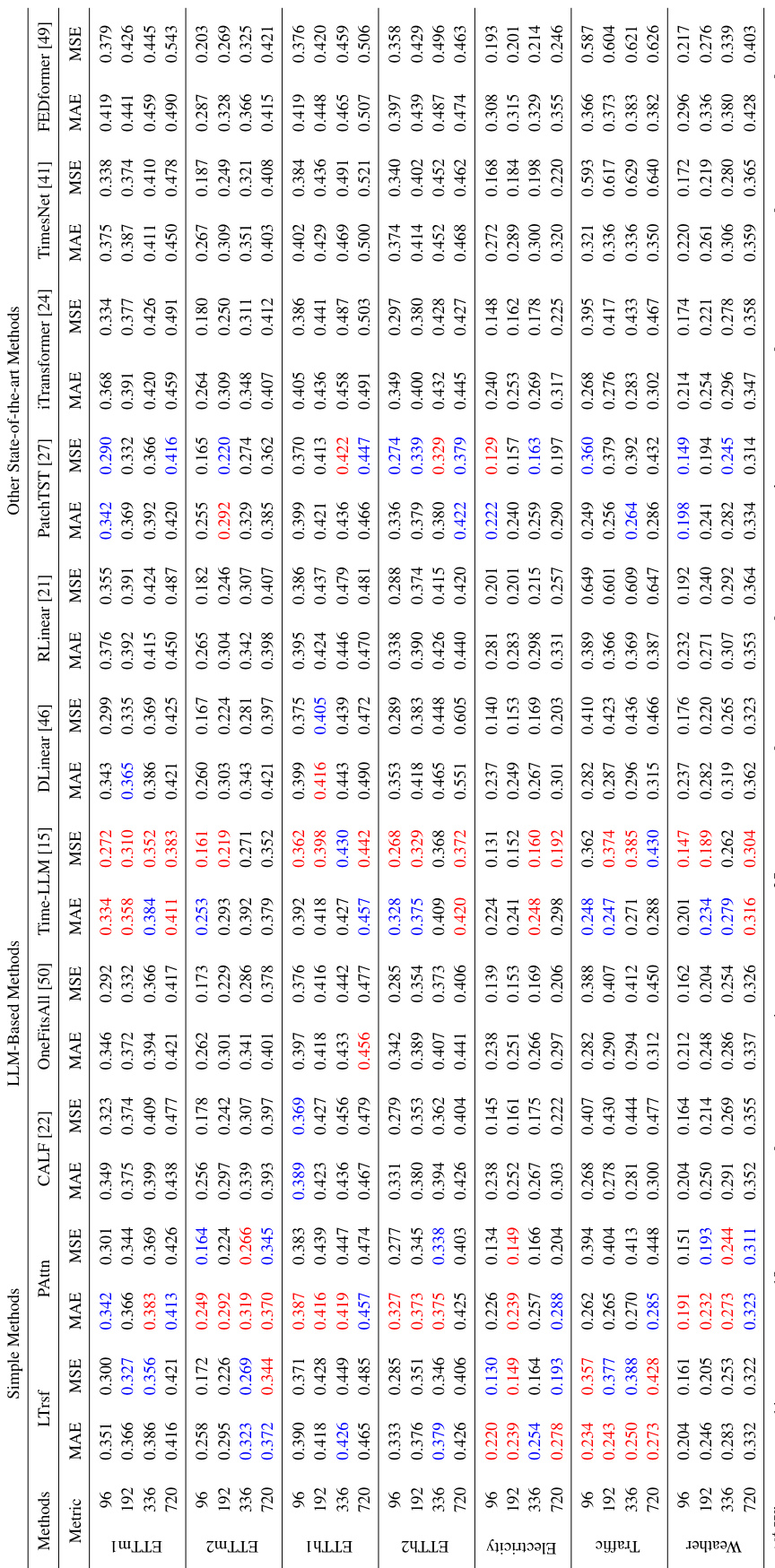
This table presents the forecasting performance (MAE and MSE) for three popular LLM-based time series forecasting methods (Time-LLM, CALF, OneFitsAll) and their corresponding ablation studies (w/o LLM, LLM2Attn, LLM2Trsf) across thirteen benchmark datasets. The results are averaged over different prediction lengths. The table highlights the best-performing method for each dataset and metric, indicating the number of times each method achieved the best performance. The number of model parameters is also included for comparison.

This table presents a comparison of the forecasting performance (MAE and MSE) of three popular LLM-based time series forecasting methods (Time-LLM, CALF, OneFitsAll) and their corresponding ablations (w/o LLM, LLM2Attn, LLM2Trsf) across thirteen datasets. The results are averaged across multiple prediction lengths. The table highlights the best-performing model for each dataset and metric and indicates the number of times each method achieved the best performance.

This table presents the forecasting performance results for three popular LLM-based time series forecasting methods (Time-LLM, CALF, OneFitsAll) and their corresponding ablation variants. The performance is evaluated using MAE and MSE metrics across thirteen benchmark datasets and four prediction lengths. The table highlights the best performing method for each dataset and metric combination and indicates the number of times each model achieved the best performance. The number of model parameters for each model is also shown.
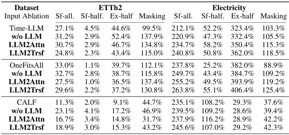
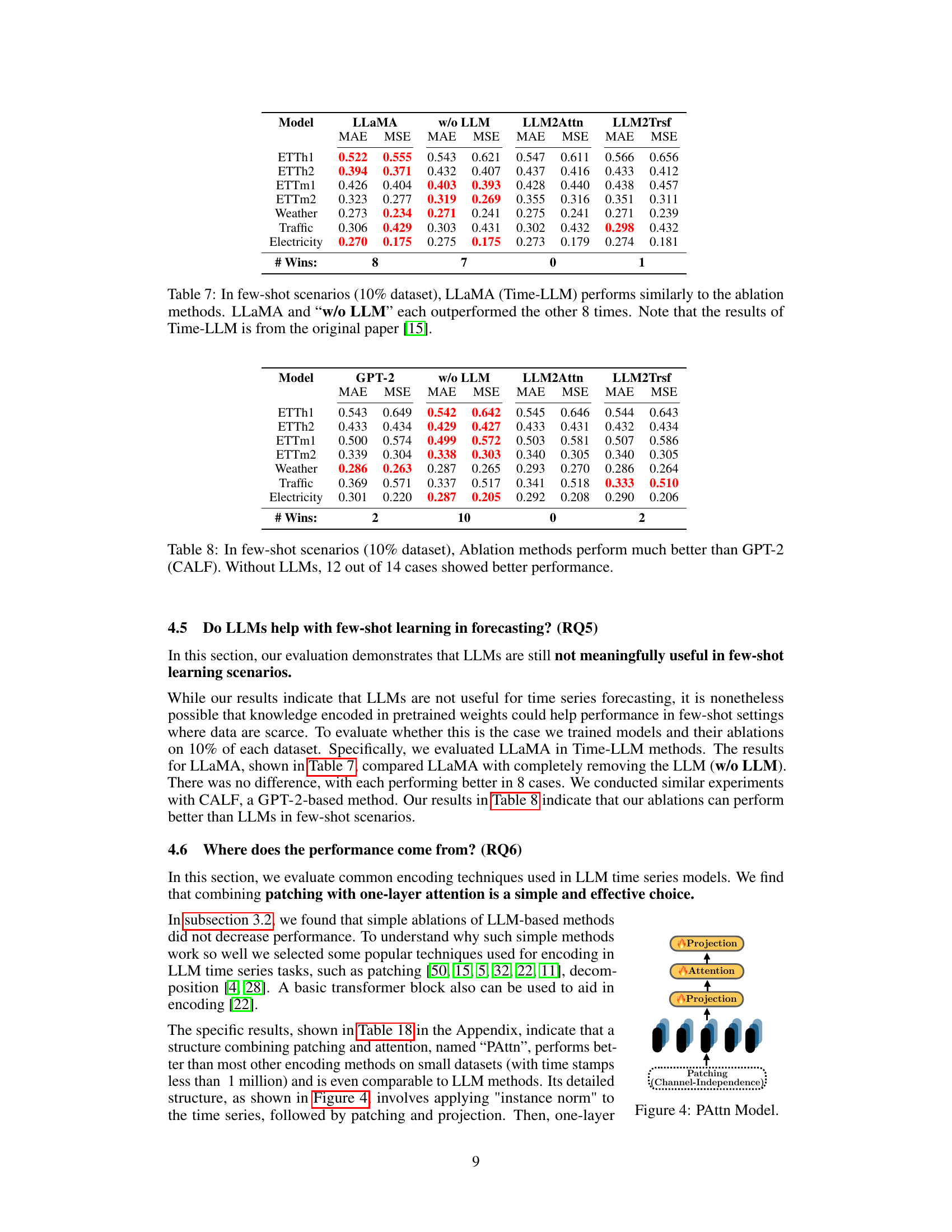
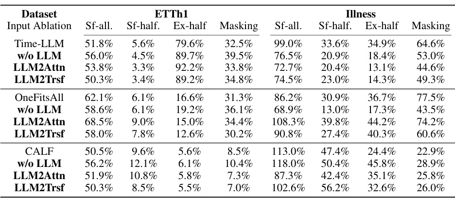
This table presents the results of experiments evaluating the effect of input shuffling and masking on the performance of three time series forecasting methods: Time-LLM, CALF, and OneFitsAll. The experiments were conducted on two datasets, ETTh1 and Illness, with various prediction lengths. The results show that shuffling or masking the input data does not significantly impact the forecasting performance, regardless of whether or not the large language model component is included in the model.

This table presents the forecasting performance results (MAE and MSE) for three popular LLM-based time series forecasting models (Time-LLM, CALF, OneFitsAll) and their corresponding ablation methods (without LLM, LLM replaced with attention, LLM replaced with transformer). Results are shown for thirteen datasets, averaged over different prediction lengths. The best performing model for each dataset and metric is highlighted in red, and the number of times each model outperformed others is also noted (# Wins). The table also shows the number of parameters used by each model.

This table presents the forecasting performance results (MAE and MSE) for three popular LLM-based time series forecasting methods (Time-LLM, CALF, OneFitsAll) and their corresponding ablation versions. The results are averaged across various prediction lengths. The table highlights the best performing model for each dataset and metric, and shows the number of times each method achieved the best performance (#Wins) and the number of model parameters (#Params). Datasets not included in the original papers are marked with ‘-’.
Full paper#

