Poisson Variational Autoencoder

↗ OpenReview ↗ NeurIPS Proc. ↗ Chat

TL;DR

#

Key Takeaways

#

Why does it matter?

#

This paper is significant because it introduces a novel architecture, the Poisson Variational Autoencoder (P-VAE), that bridges the gap between artificial neural networks and neuroscience. The P-VAE’s design, incorporating principles of predictive coding and Poisson-distributed latent variables, offers a more biologically plausible model for sensory processing. This has implications for improving the interpretability and efficiency of deep learning models and for advancing our understanding of the brain’s mechanisms for perception. The model’s ability to avoid posterior collapse and achieve high sample efficiency in downstream tasks is particularly noteworthy. The findings pave the way for more biologically inspired and efficient AI models and a deeper understanding of perception as an inferential process.

Visual Insights

#

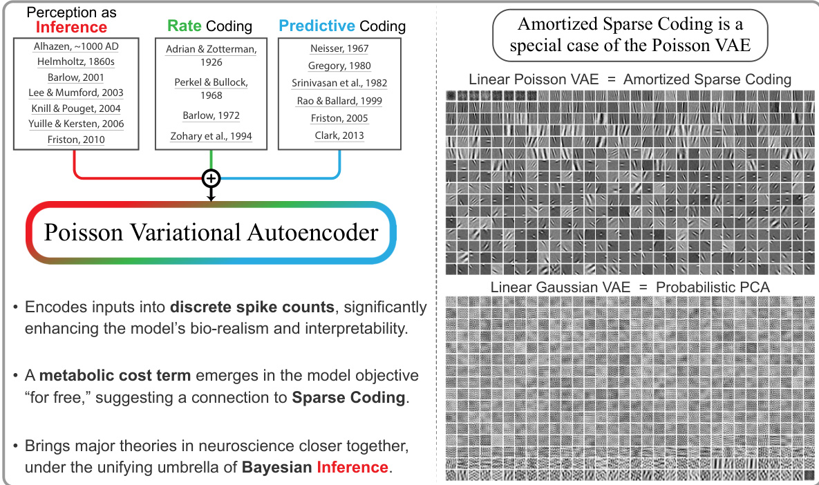
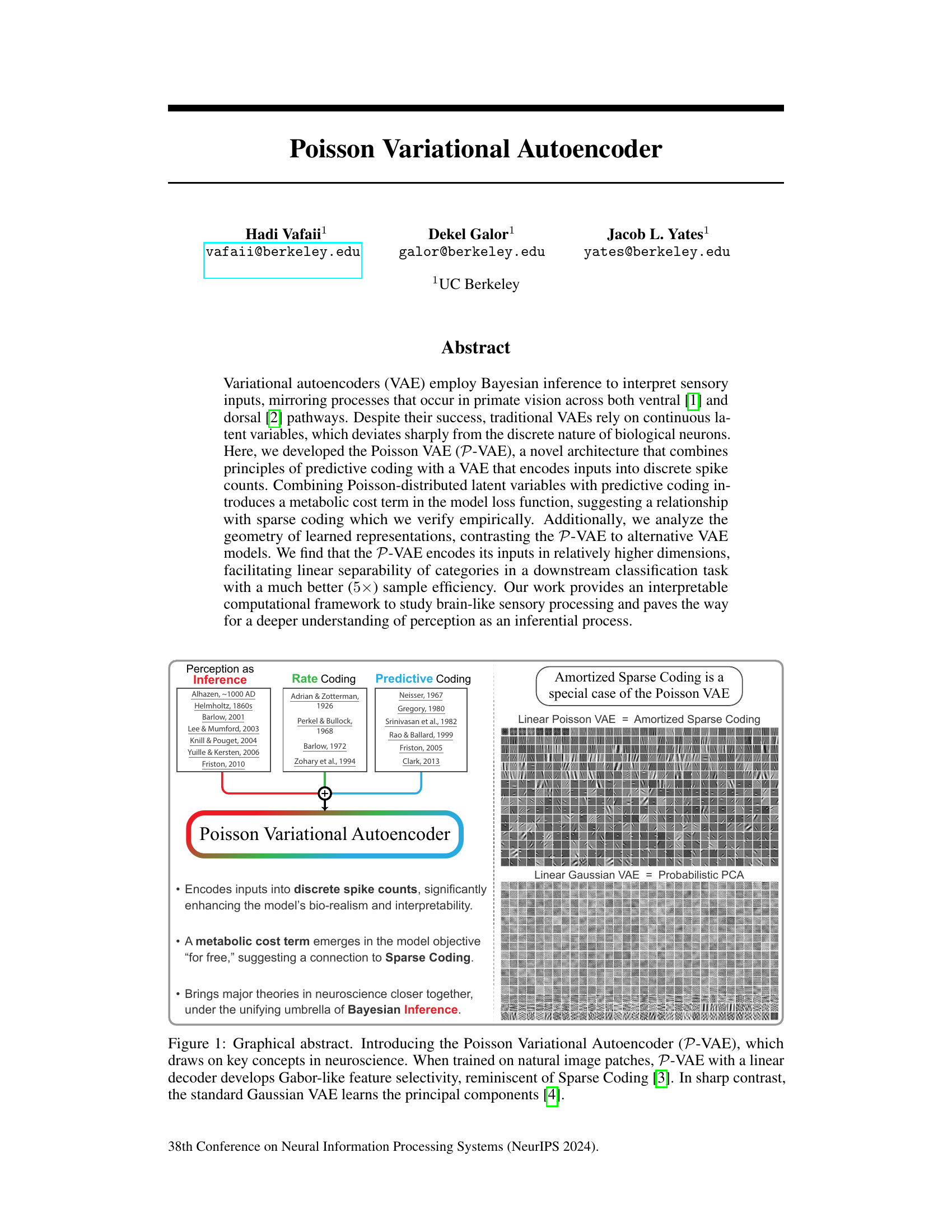
This figure is a graphical abstract that introduces the Poisson Variational Autoencoder (P-VAE). It highlights the model’s key features: encoding inputs as discrete spike counts, incorporating a metabolic cost term linking to sparse coding, and unifying major neuroscience theories under Bayesian inference. The figure contrasts the P-VAE’s Gabor-like feature learning with the principal component analysis of standard Gaussian VAEs when trained on natural images.

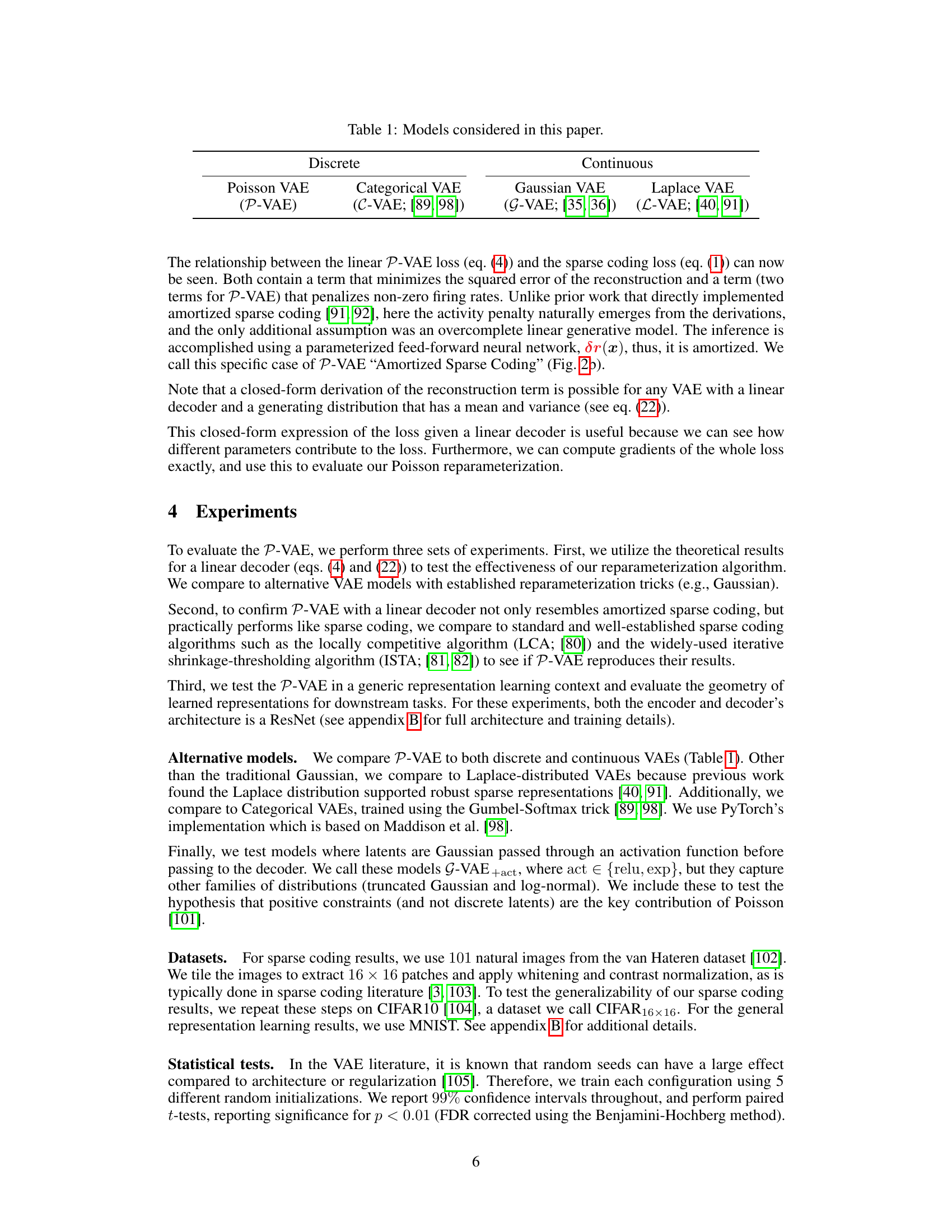
This table summarizes the different variational autoencoder (VAE) models used in the paper for comparison purposes. It highlights whether the model utilizes a discrete or continuous latent space, and provides references for each model. The models include the Poisson VAE (P-VAE), the Categorical VAE (C-VAE), the Gaussian VAE (G-VAE), and the Laplace VAE (L-VAE).

In-depth insights

#

Poisson VAE Model

#

The Poisson Variational Autoencoder (P-VAE) model presents a novel approach to variational autoencoders by incorporating Poisson-distributed latent variables. This design choice is motivated by the biological realism of representing neural activity as discrete spike counts, rather than continuous values. A key advantage of the P-VAE is its inherent connection to sparse coding, which emerges naturally from the model’s objective function and the inclusion of a metabolic cost term. This metabolic cost term reflects a biological constraint on neural energy and promotes sparse representations. Further, the P-VAE demonstrates improved performance in a classification task, showcasing a significant increase in sample efficiency. The incorporation of predictive coding principles enhances the model’s interpretability and alignment with biological processes. By modeling inputs as deviations from prior expectations, the P-VAE provides a computational framework for studying brain-like sensory processing and improves representation learning.

Sparse Coding Link

#

The concept of a ‘Sparse Coding Link’ within the context of a variational autoencoder (VAE) framework suggests a connection between the model’s learned representations and the principles of sparse coding in neuroscience. Sparse coding emphasizes representing data with a minimal number of active elements, promoting efficiency and interpretability. A successful ‘Sparse Coding Link’ in a VAE would manifest in the model learning latent representations that are sparse, meaning most latent variables are inactive or near zero for any given input. This would align with biological neural networks, where only a small subset of neurons fire in response to a stimulus. Establishing this link could have several implications, including improved model interpretability by relating latent variables to specific features, increased efficiency in data representation, and a stronger connection between artificial and biological neural systems. The key would be demonstrating that the VAE’s learned latent space exhibits properties consistent with sparse coding, such as sparse activation patterns and efficient encoding of input information. This could involve analyzing the distribution of latent variable activations, comparing the learned features to those found in biological visual systems (e.g., Gabor filters), and assessing the model’s performance against known sparse coding algorithms.

Amortized Inference

#

Amortized inference is a crucial concept in variational autoencoders (VAEs), significantly impacting efficiency and scalability. Instead of performing inference separately for each data point, amortized inference trains a neural network, the inference network, to approximate the posterior distribution for any given input. This avoids computationally expensive repeated calculations, making the VAE significantly faster. The inference network learns a mapping from the input space to the latent space, effectively encoding this mapping. A key advantage is improved sample efficiency in downstream tasks; having pre-computed the mapping, the model is faster to use. However, amortized inference is not without limitations. The inference network must generalize well to unseen data, and limitations in its capacity can lead to poor approximations of the true posterior, ultimately affecting the model’s performance. The trade-off between accuracy of posterior approximation and computational speed inherent in amortized inference is a key consideration in VAE design. Furthermore, posterior collapse, a common issue in VAEs, can be exacerbated by limitations in the capacity of the inference network. This highlights the delicate balance that must be struck during model design.

Posterior Collapse

#

Posterior collapse in variational autoencoders (VAEs) is a critical issue where the learned latent representation fails to capture the full diversity of the input data. Instead, the model’s posterior distribution over latent variables collapses, becoming overly concentrated, often around a single point. This severely limits the VAE’s ability to generate diverse outputs and hinders its effectiveness as a generative model. The root cause often lies in the KL divergence term of the VAE’s loss function, which penalizes the difference between the learned posterior and the prior. If this penalty is too strong, it forces the posterior to closely match the prior, regardless of the input data, leading to the collapse. Several techniques have been proposed to mitigate posterior collapse, including using larger latent spaces, modifying the KL term (e.g., using a different annealing schedule), employing different prior distributions (e.g., more complex priors than simple Gaussians), and incorporating architectural changes such as implementing a discrete latent space. Understanding and addressing posterior collapse is crucial for building effective VAEs capable of learning meaningful and diverse representations of complex data.

Future Directions

#

The study’s ‘Future Directions’ section would ideally delve into extending the Poisson VAE (P-VAE) to handle hierarchical structures, mirroring the brain’s hierarchical organization. This could involve exploring how conditional Poisson distributions could model spike trains more realistically. Addressing the amortization gap between P-VAE and traditional sparse coding methods is another crucial area. This could involve investigating more expressive encoder architectures or exploring alternative inference techniques like iterative methods to improve approximation accuracy. Further research should explore the impact of different activation functions beyond the sigmoid and address how P-VAE scales to larger, more complex datasets. Finally, investigating the potential applications of P-VAE in modeling other brain regions or sensory modalities beyond vision would significantly broaden its impact, showcasing the generalizability and flexibility of this novel approach. The biological realism of the model’s design suggests it could be adapted for studying other neurobiological phenomena and offer valuable insights into brain function.

More visual insights

#

More on figures

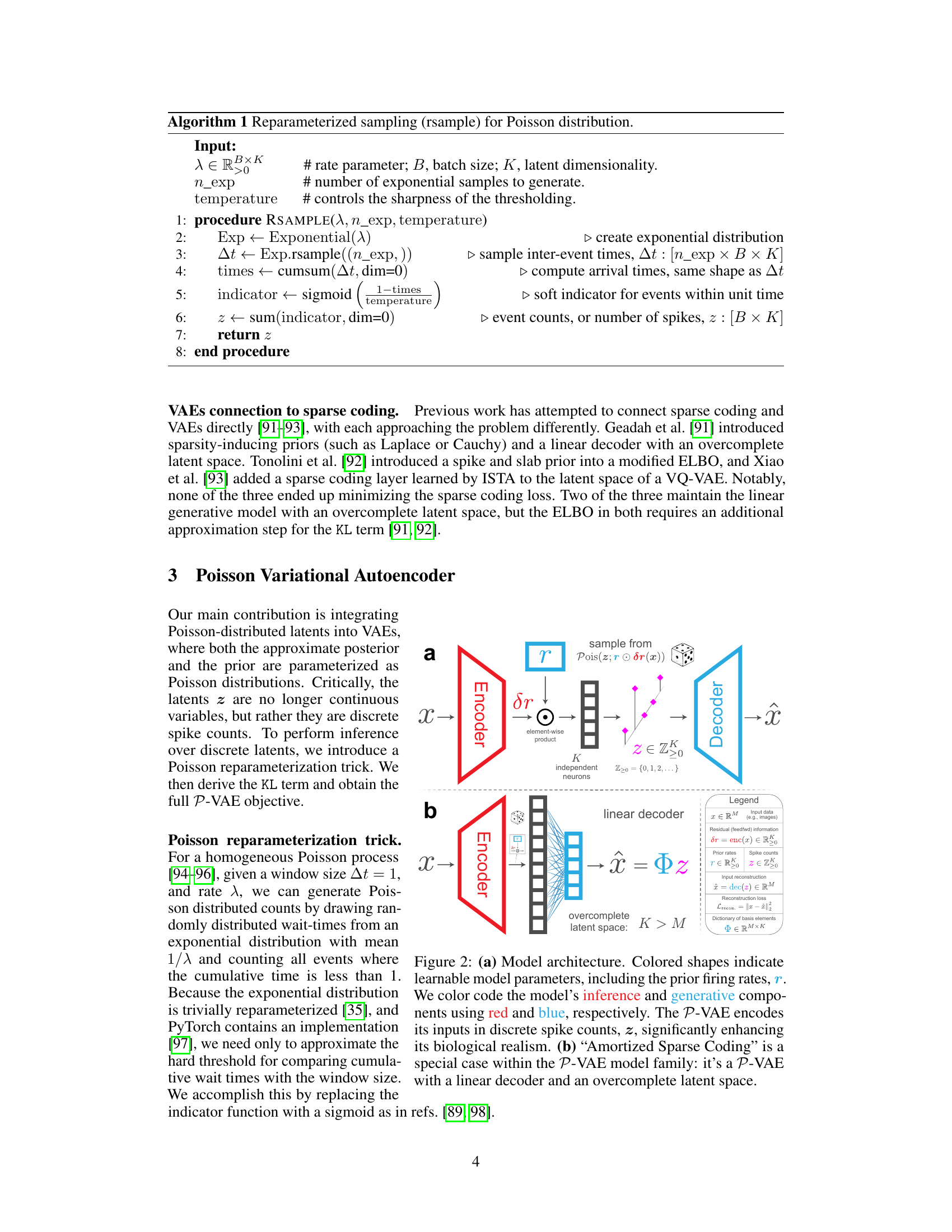
Figure 2 illustrates the architecture of the Poisson Variational Autoencoder (P-VAE). Panel (a) shows the general structure, highlighting the encoder (red), decoder (blue), and the process of encoding inputs into discrete spike counts. Panel (b) focuses on a special case of the P-VAE, named ‘Amortized Sparse Coding’, featuring a linear decoder and an overcomplete latent space.

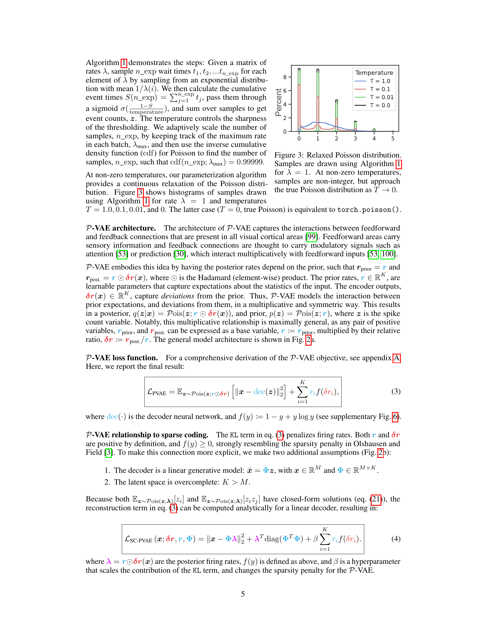
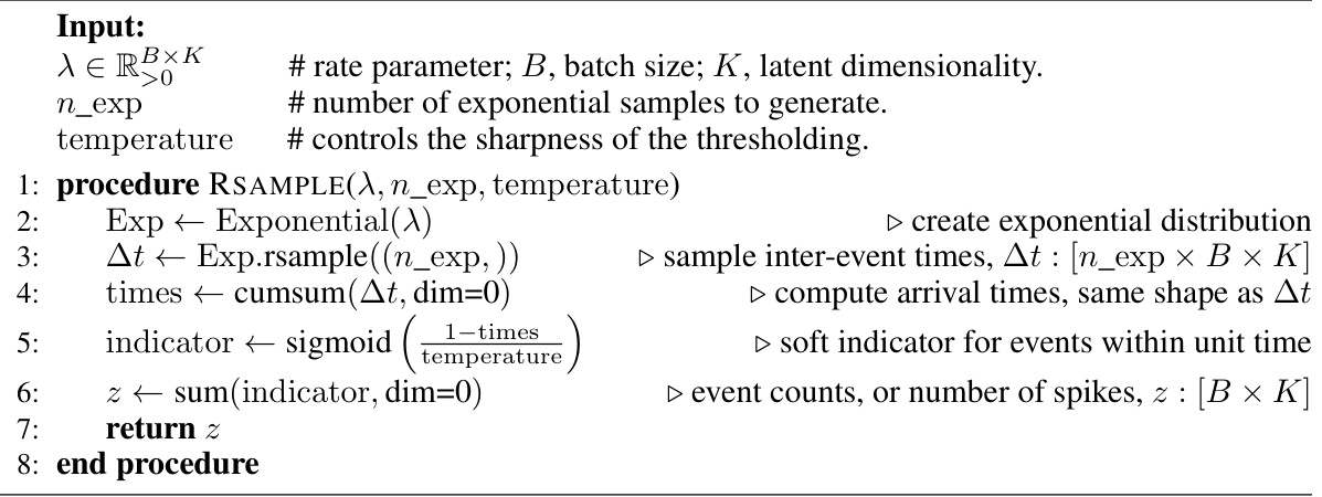
This figure shows the effect of temperature parameter in Algorithm 1 on the generated Poisson distribution. Algorithm 1 uses a reparameterization trick to sample from a Poisson distribution. The temperature parameter controls the sharpness of the thresholding function within the algorithm. As the temperature approaches zero, the resulting distribution more closely resembles a true Poisson distribution, with non-integer values present at non-zero temperatures. The figure contains four plots, one each for T = 1.0, T = 0.1, T = 0.01, and T = 0.0.

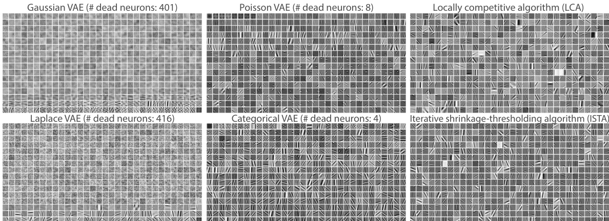
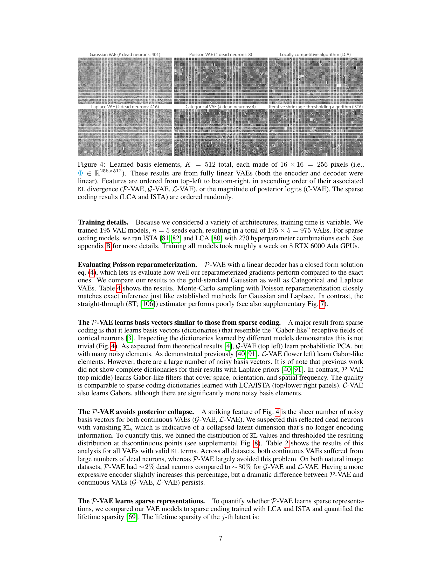
This figure compares the learned basis elements (dictionary) from different VAE models and sparse coding algorithms. Each image represents a basis element. The ordering of the VAE basis elements are determined by their KL divergence value, while the sparse coding results are ordered randomly. The figure visually demonstrates that P-VAE learns basis elements that closely resemble the Gabor-like receptive fields found in the visual cortex, similar to sparse coding.

This figure shows the learned basis elements (dictionary) for several VAE models, including the Poisson VAE, compared to sparse coding methods. It highlights that the Poisson VAE with a linear decoder learns Gabor-like filters, similar to sparse coding algorithms, while other VAEs (Gaussian, Laplace, Categorical) show more noise and less organized structure. The arrangement of the basis elements reflects the order of their KL divergence or logit magnitude.

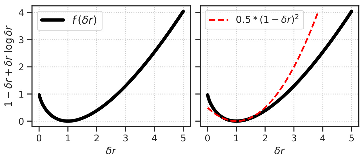
The figure shows two plots. The left plot shows the residual term f(δr) = 1 - δr + δr log δr as a function of δr. The right plot shows a quadratic approximation of f(δr), which is 0.5 * (1 - δr)^2, along with the actual f(δr) function for comparison. These plots illustrate the behavior of the KL term in the Poisson VAE loss function, particularly how it penalizes deviations from the prior firing rate.

This figure compares the learned basis elements (dictionary) from different VAE models (P-VAE, G-VAE, L-VAE, C-VAE) and sparse coding methods (LCA, ISTA) trained on natural image patches. Each basis element is a 16x16 pixel image. The ordering of the elements is based on either the KL divergence (for continuous VAEs) or the magnitude of posterior logits (for C-VAE). The comparison highlights the differences in the learned representations: P-VAE learns Gabor-like features similar to sparse coding, while other VAEs show less interpretable, more noisy features. This suggests P-VAE’s ability to learn biologically plausible representations.

This figure compares the learned basis elements (dictionary) from different VAE models with those obtained from sparse coding algorithms. The P-VAE learns Gabor-like features, similar to those observed in the visual cortex and obtained by sparse coding methods. In contrast, the Gaussian VAE learns principal components, and the Laplace VAE learns a mixture of Gabor-like and noisy features. The categorical VAE also learns Gabor-like features, but with more noise.

This figure compares the learned basis elements (filters) from different VAE models (Poisson VAE, Gaussian VAE, Laplace VAE, Categorical VAE) and sparse coding methods (LCA, ISTA). The filters from linear decoders, which are ordered based on their KL divergence or logit magnitudes, show the ability of the Poisson VAE to learn Gabor-like features, similar to sparse coding, unlike the others which learn noisy elements or principal components. The image clearly demonstrates the P-VAE’s capacity for learning biologically plausible features compared to other VAE models.

More on tables

This table presents four different variational autoencoder (VAE) models used for comparison in the paper. Two are discrete VAEs (Poisson VAE and Categorical VAE), and two are continuous VAEs (Gaussian VAE and Laplace VAE). The table lists the name of each model and relevant citations to prior work where those models were introduced.

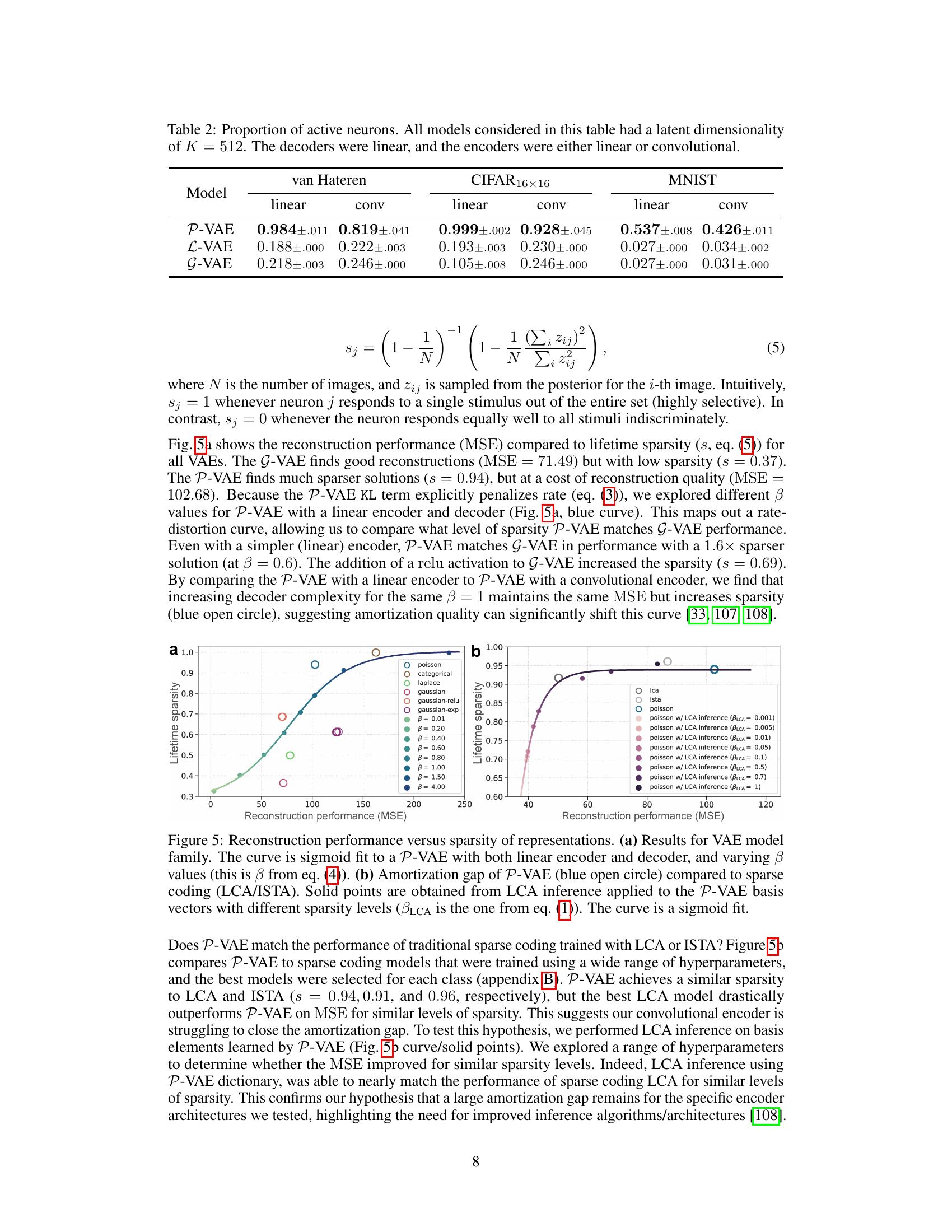
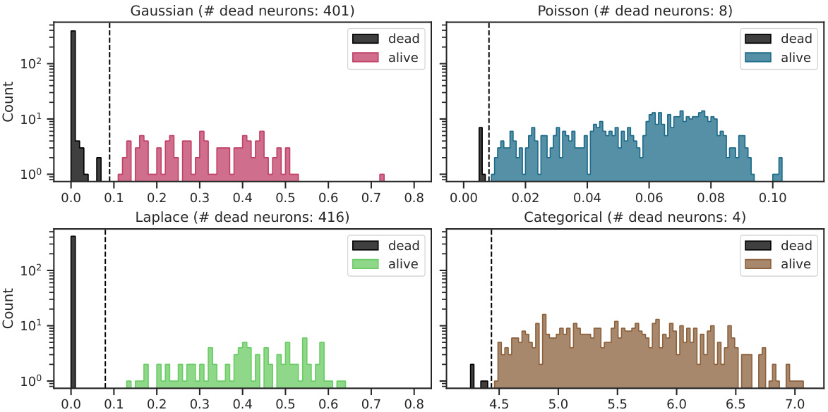
This table shows the proportion of active neurons for different VAE models. A high proportion indicates that the model is effectively using the latent dimensions, while a low proportion suggests posterior collapse. The results are broken down by dataset (van Hateren, CIFAR16x16, MNIST) and encoder type (linear, convolutional).

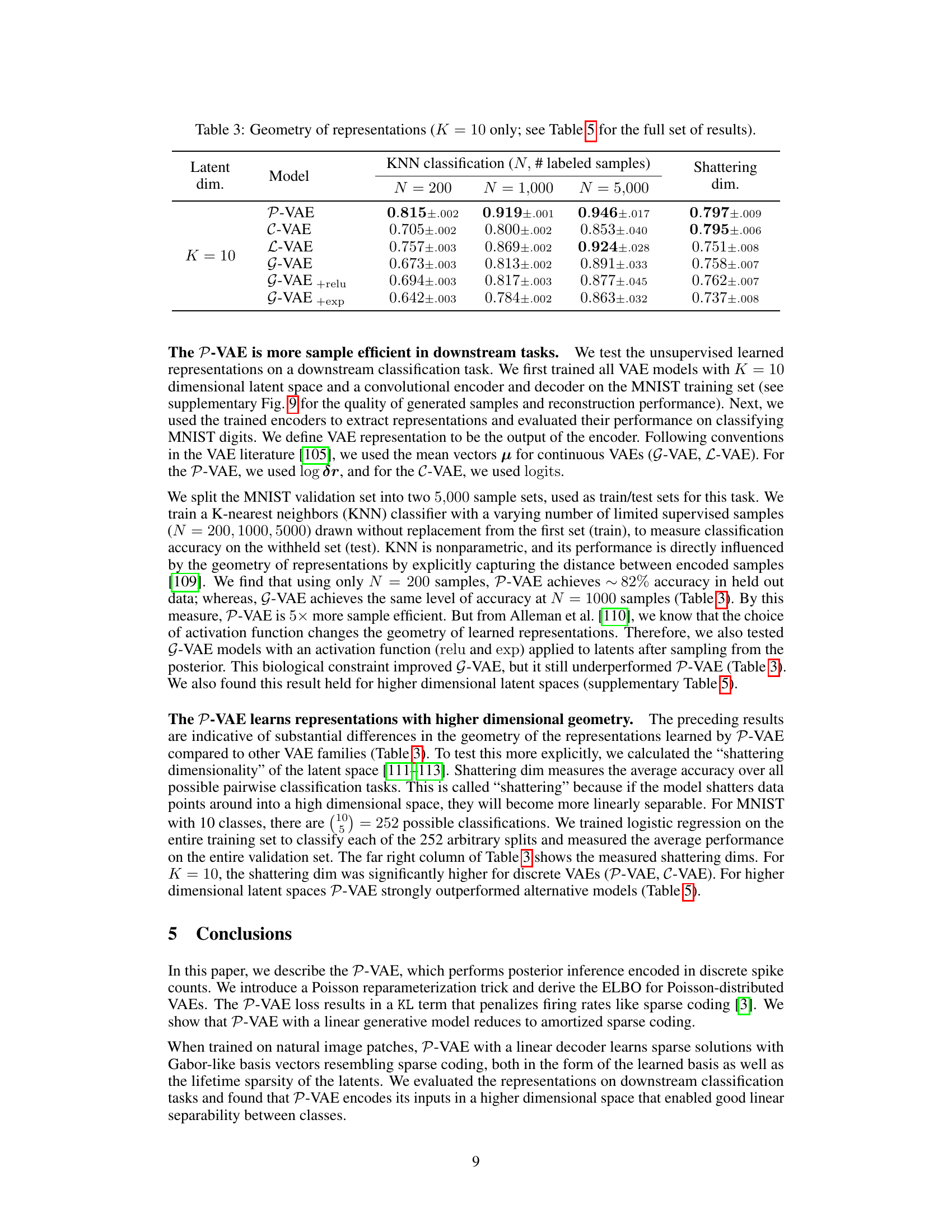
This table presents the results of a K-Nearest Neighbors (KNN) classification task performed on unsupervised learned representations from various VAE models. The goal is to assess the sample efficiency and geometric properties of the different latent spaces in a downstream classification task. The table shows the accuracy of KNN classification for different numbers of labeled samples (N = 200, 1000, 5000) and also includes the ‘shattering dimension’, which measures the linear separability of the learned representations. A higher shattering dimension generally indicates better linear separability.

This table shows the proportion of active neurons for different VAE models. A ‘dead neuron’ indicates a latent dimension that is not actively encoding information, a phenomenon known as posterior collapse. The table compares the performance of the Poisson VAE (P-VAE) against other continuous and discrete VAE models (G-VAE, L-VAE, and C-VAE) across different datasets (van Hateren, CIFAR16x16, and MNIST) and encoder architectures (linear and convolutional). Lower numbers indicate fewer dead neurons and thus better performance.

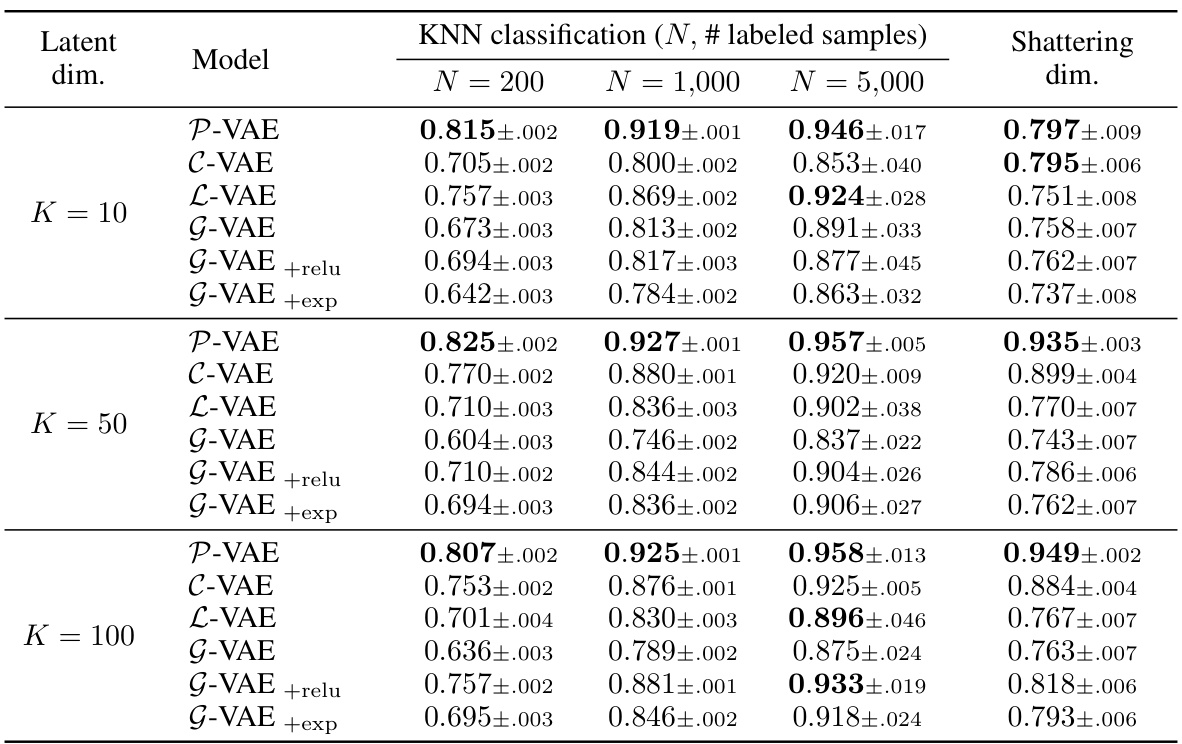
This table presents the results of a downstream classification task using K-Nearest Neighbors (KNN) with different numbers of labeled samples (N = 200, 1000, 5000). The task is to classify MNIST digits using feature representations learned by various VAE models (P-VAE, C-VAE, L-VAE, G-VAE, G-VAE+relu, G-VAE+exp) with a latent dimensionality of K=10. The table shows the accuracy of each model for each sample size (N), and also includes the ‘shattering dimension’, which measures the average accuracy over all possible pairwise classification tasks. This provides insight into the geometry of the learned representations and how well the models generalize to different classification tasks.

Full paper

#