↗ OpenReview ↗ NeurIPS Proc. ↗ Chat
TL;DR#
Current climate models are computationally expensive, limiting the exploration of various climate scenarios. Data-driven surrogates, though promising, often struggle with long-term simulations. This paper tackles these challenges by presenting a novel approach.
The proposed method, Spherical DYffusion, integrates the dynamics-informed diffusion framework with Spherical Fourier Neural Operators. This combination enables stable, 100-year simulations at 6-hourly timesteps with low computational cost. The model demonstrates high accuracy in emulating a real-world climate model, exceeding the performance of existing baselines and showing improved skill in generating climate ensembles, crucial for uncertainty quantification.
Key Takeaways#
Why does it matter?#
This paper is crucial because it presents the first generative model for probabilistic climate simulation, overcoming limitations of existing deterministic approaches. It offers improved accuracy and efficiency, paving the way for more sophisticated climate modeling and better uncertainty quantification. This opens avenues for ensemble climate projections crucial for climate change research and policymaking. The efficient method allows for more extensive exploration of climate scenarios and improved risk assessment.
Visual Insights#
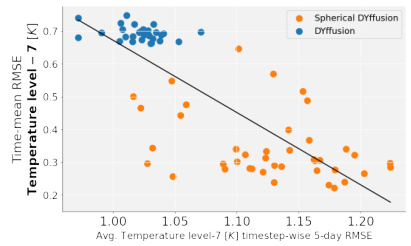
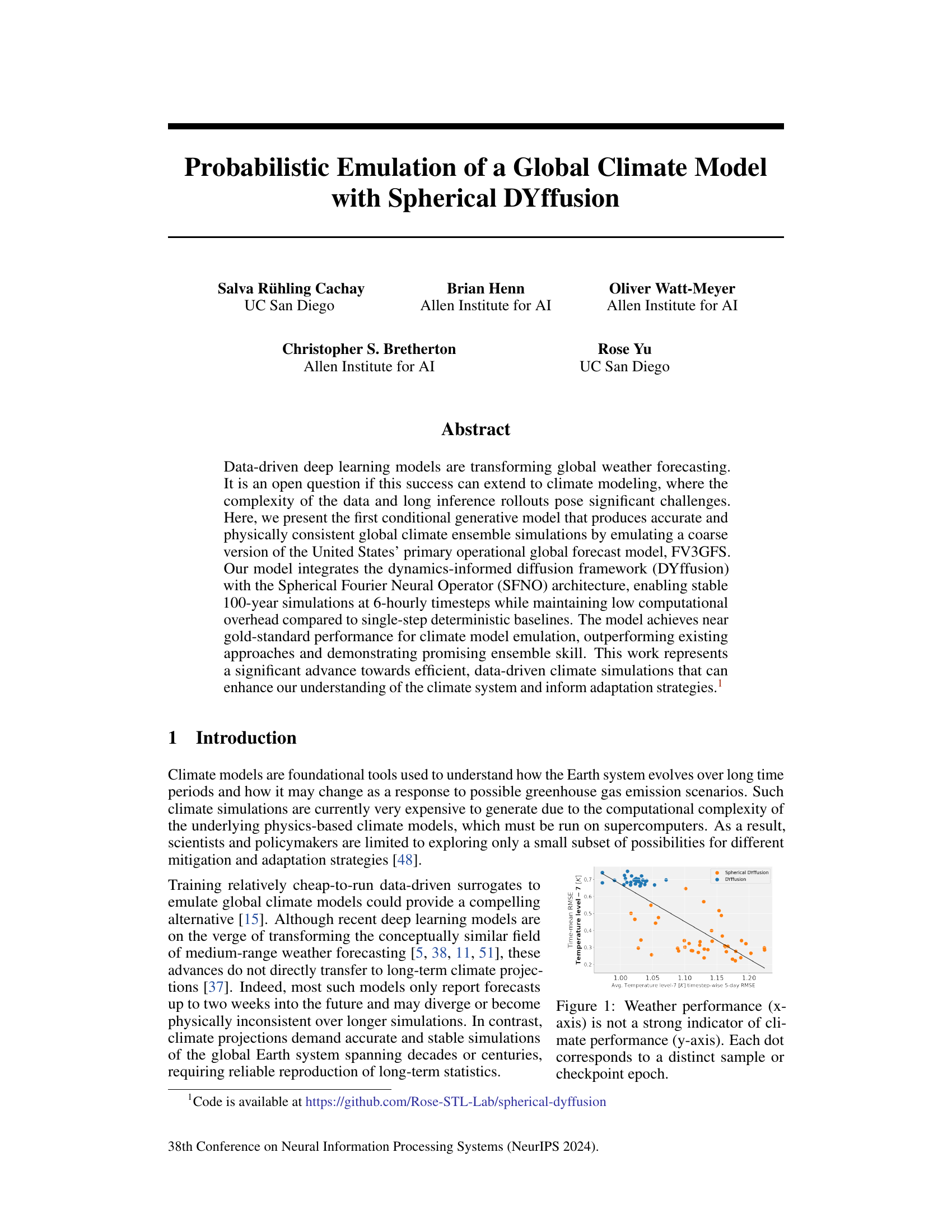
This figure shows the divergence between medium-range weather forecasting skill and longer-term climate performance. The x-axis represents the average RMSE of 5-day weather forecasts, while the y-axis shows the RMSE of the 10-year time-mean climate simulations. Each point represents a distinct model sample or checkpoint epoch. The lack of correlation between the two metrics highlights that good short-term weather forecasts do not necessarily guarantee good long-term climate simulations. Small, systematic errors in short-term predictions can accumulate over time and lead to large biases in long-term climate statistics.
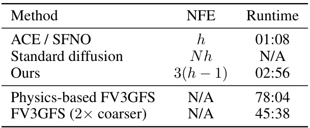
This table compares the computational complexity of different deep learning models for climate prediction, measured by the number of neural network forward passes (NFEs) and the total inference time for a 10-year simulation. It shows that the proposed Spherical DYffusion method is significantly more computationally efficient than standard diffusion models and comparable to deterministic baselines, while still achieving high accuracy.
In-depth insights#
Spherical DYffusion#
The proposed model, Spherical DYffusion, is a novel approach that integrates the strengths of two powerful frameworks: the dynamics-informed diffusion model (DYffusion) and the Spherical Fourier Neural Operator (SFNO). DYffusion’s generative nature enables probabilistic climate simulations, crucial for uncertainty quantification, while SFNO’s efficiency handles the high dimensionality of spherical climate data. This combination overcomes limitations of previous methods, allowing for stable, physically consistent, and computationally efficient 100-year climate simulations. A key innovation is the incorporation of time conditioning and inference stochasticity into the SFNO architecture, improving the model’s ability to capture long-term climate dynamics. The results show that Spherical DYffusion outperforms existing approaches, demonstrating reduced climate biases and improved ensemble skill. Importantly, the work highlights that good short-term weather forecasting skill does not guarantee accurate long-term climate predictions, emphasizing the unique challenges and opportunities in ML-based climate modeling.
Climate Model Emulation#
Climate model emulation uses machine learning to create more efficient surrogates for computationally expensive climate models. This approach offers significant advantages, including faster simulations, the ability to explore a wider range of scenarios, and reduced computational costs. The core challenge lies in balancing accuracy and computational efficiency; models must accurately reproduce the complex dynamics of the climate system while remaining computationally tractable. Generative models are particularly promising as they can capture the inherent uncertainty in the climate system and produce physically consistent ensembles. However, successful emulation requires careful consideration of the model architecture, training data, and evaluation metrics, as the success of these surrogates is highly dependent on all three. Further research will likely involve addressing biases in emulated models, enhancing their stability for long-term projections and improving the representation of uncertainty to better inform adaptation and mitigation strategies.
Ensemble Climate#
The concept of ‘Ensemble Climate’ in climate modeling refers to the generation and analysis of multiple climate simulations, each run with slightly different initial conditions or parameterizations. This approach is crucial because climate systems are inherently chaotic, meaning that small variations in initial states can lead to significantly different long-term outcomes. An ensemble approach mitigates this uncertainty by providing a range of possible future climate scenarios, offering a more comprehensive understanding than any single simulation. Analyzing the spread and distribution of model results within an ensemble allows for better quantification of uncertainty and identification of robust features that persist across the various runs, improving our understanding of the relative importance of internal variability versus external forcing factors in driving climate change. Probabilistic approaches, such as those based on diffusion models, are particularly well-suited to generating and analyzing climate ensembles, as they naturally capture the inherent uncertainties and probability distributions involved in these systems. The use of ensembles aids decision-making by providing a clearer picture of potential future climate states, thus aiding in developing more robust adaptation and mitigation strategies.
DYffusion Framework#
The DYffusion framework represents a significant advancement in diffusion models, particularly for sequential data like time series. By directly incorporating temporal dynamics, it overcomes limitations of standard diffusion models that struggle with long sequences. The framework’s core innovation is its dynamics-informed approach. Instead of relying solely on denoising, DYffusion cleverly interweaves a forward process (temporal interpolation) with a reverse process (forecasting). This dual approach allows for more efficient sampling and enhanced accuracy, especially crucial for computationally expensive climate modeling. The low computational overhead at inference time is a key feature, making it highly practical for real-world applications. However, the original DYffusion model’s reliance on U-Net architecture, which is better suited to Euclidean data, limits its applicability to spherical data. Addressing this limitation is essential for expanding its utility in geospatial domains like climate modeling.
SFNO Architecture#
The Spherical Fourier Neural Operator (SFNO) architecture is a crucial component of the research, offering a powerful mechanism for efficiently processing and modeling spherical data such as global climate information. SFNO leverages the Spherical Fourier Transform, which is computationally efficient and naturally handles spherical symmetries. This is a significant advantage over traditional methods that struggle with the inherent complexities of spherical geometry. SFNO’s ability to model long-range dependencies in the data is critical for simulating climate phenomena that evolve over extended periods. By operating in the Fourier domain, SFNO captures global patterns and interactions efficiently, avoiding the computational burden of explicitly modeling local interactions across vast datasets. The integration of SFNO with the dynamics-informed diffusion model (DYffusion) framework is a key innovation, combining the strengths of each approach to yield accurate and stable long-term climate simulations. The resulting hybrid model (Spherical DYffusion) benefits from both the efficient global modeling capability of SFNO and the probabilistic sampling approach of DYffusion, paving the way for more comprehensive and reliable data-driven climate modeling.
More visual insights#
More on figures

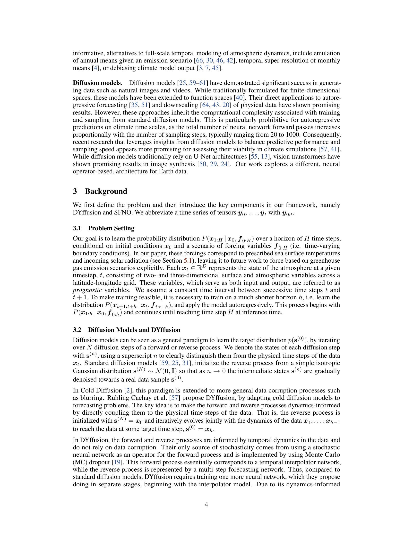
The figure displays a comparison of the 10-year time-mean RMSE for various fields between the proposed model and multiple baselines, including the reference FV3GFS simulations. It highlights the reduction in climate biases achieved by the proposed model compared to existing methods, especially when using ensemble predictions.
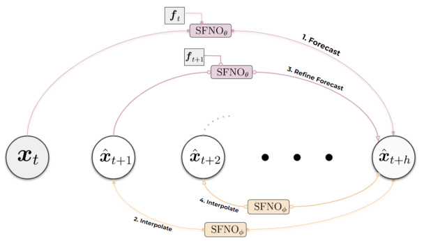
This figure illustrates the inference process of the Spherical DYffusion model. It starts with an initial condition (xt) and forcing data (ft:t+h). The model alternates between a direct multi-step forecast using SFNOθ and temporal interpolation using SFNOφ to generate predictions for the next h time steps. The process repeats recursively to make long-term predictions.
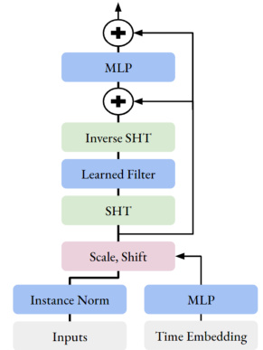
This figure shows the architecture of one block of the modified Spherical Fourier Neural Operator (SFNO) used in the proposed Spherical DYffusion model. The full model uses 8 of these blocks sequentially. The diagram highlights the addition of a new time-conditioning module, consisting of a time embedding followed by a multi-layer perceptron (MLP) that modifies the scale and shift parameters. The use of dropout within a two-layer MLP is also shown. This is compared to a standard SFNO which lacks the time embedding.

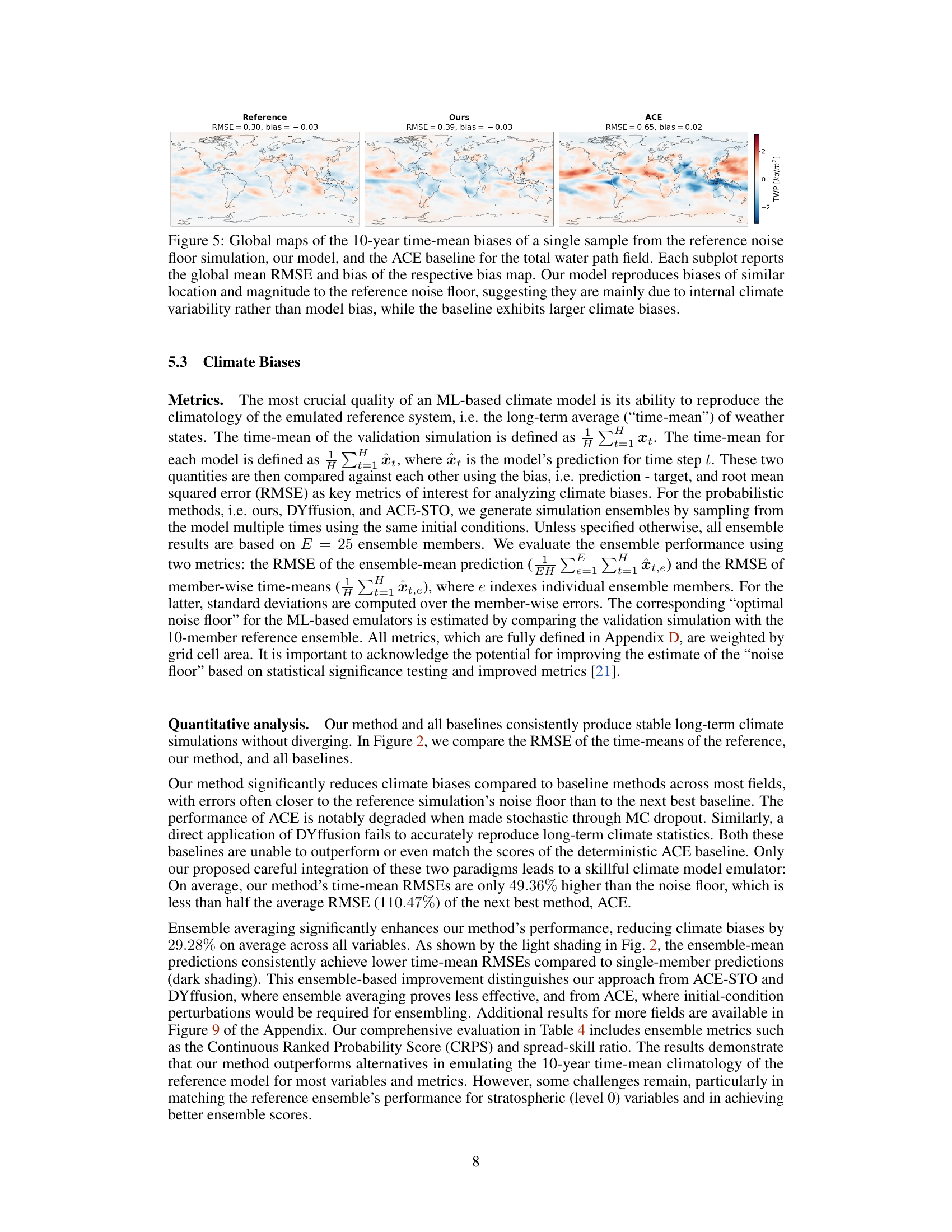
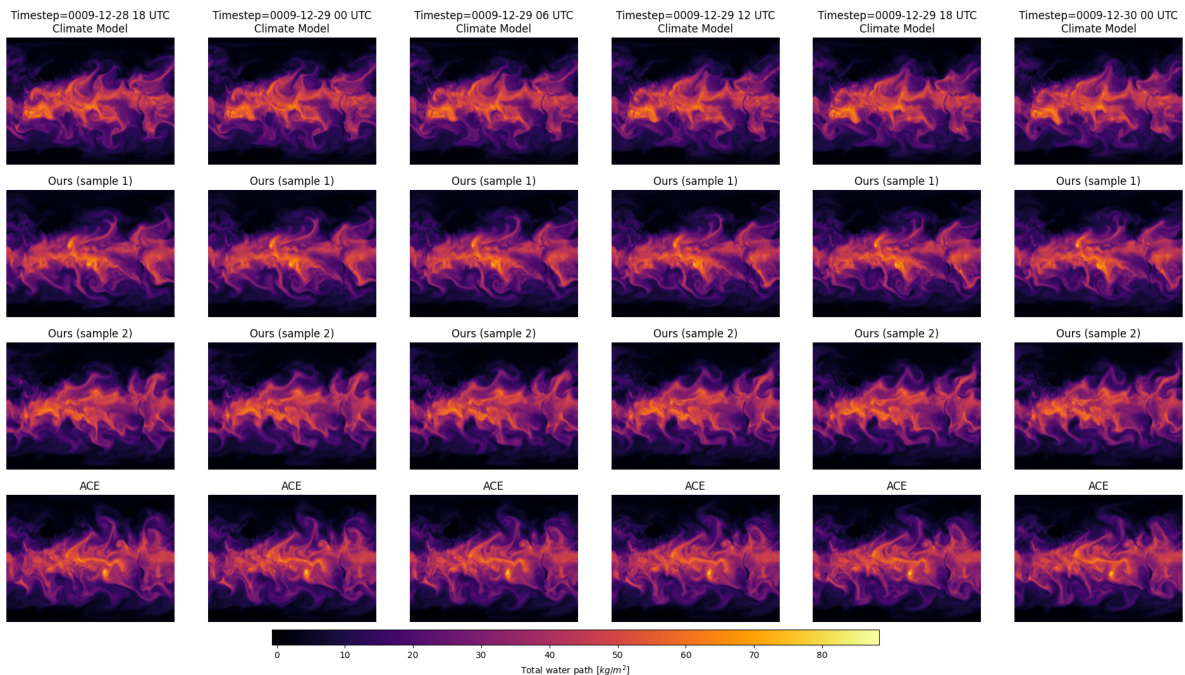
This figure displays global maps of 10-year time-mean biases for the total water path (TWP) variable, comparing the reference noise floor simulation, the proposed Spherical DYffusion model, and the ACE baseline model. The maps show spatial patterns of biases, with numerical values (RMSE and bias) provided for each model. The key finding is that Spherical DYffusion produces biases similar in location and magnitude to the noise floor, implying that the model’s errors mainly stem from inherent climate variability rather than systematic biases. In contrast, ACE demonstrates larger and more significant biases.
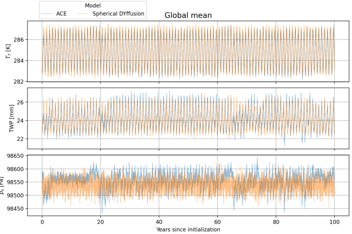
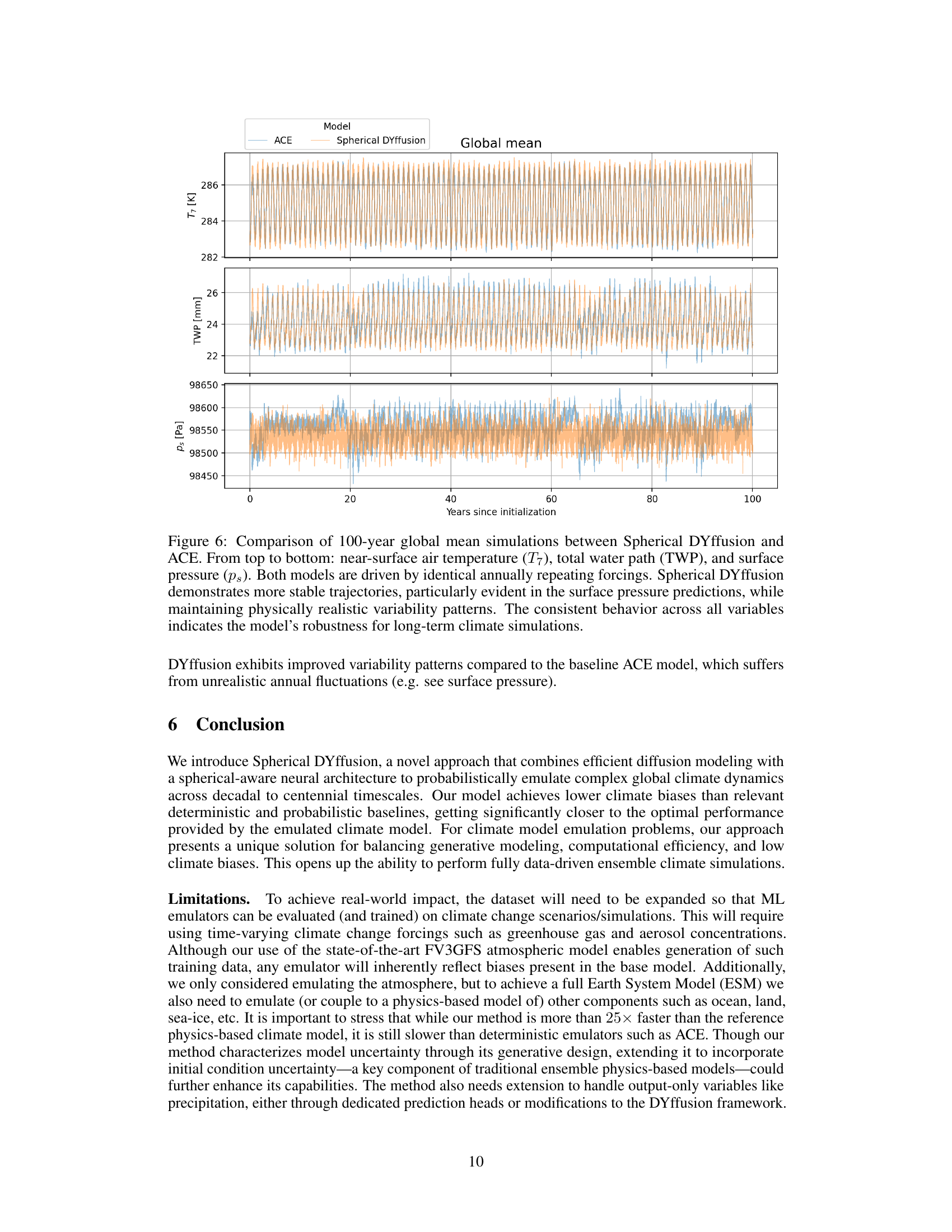
This figure compares the 100-year global mean simulations of Spherical DYffusion and ACE, driven by identical annually repeating forcings. It displays time series of near-surface air temperature (T7), total water path (TWP), and surface pressure (ps). Spherical DYffusion shows more stable trajectories than ACE, particularly in surface pressure, while maintaining realistic variability. The figure highlights Spherical DYffusion’s robustness for long-term climate simulations.
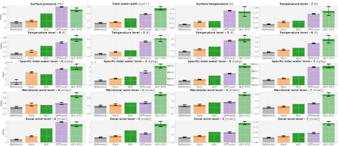
This figure compares the root mean square error (RMSE) of 10-year time-means for several important climate variables. It shows the performance of the proposed Spherical DYffusion model against several baselines (ACE, DYffusion, ACE-STO), with the reference noise floor also included. The figure highlights that Spherical DYffusion achieves lower RMSE values than the baselines, particularly when using an ensemble prediction, demonstrating its superior skill in emulating long-term climate statistics.
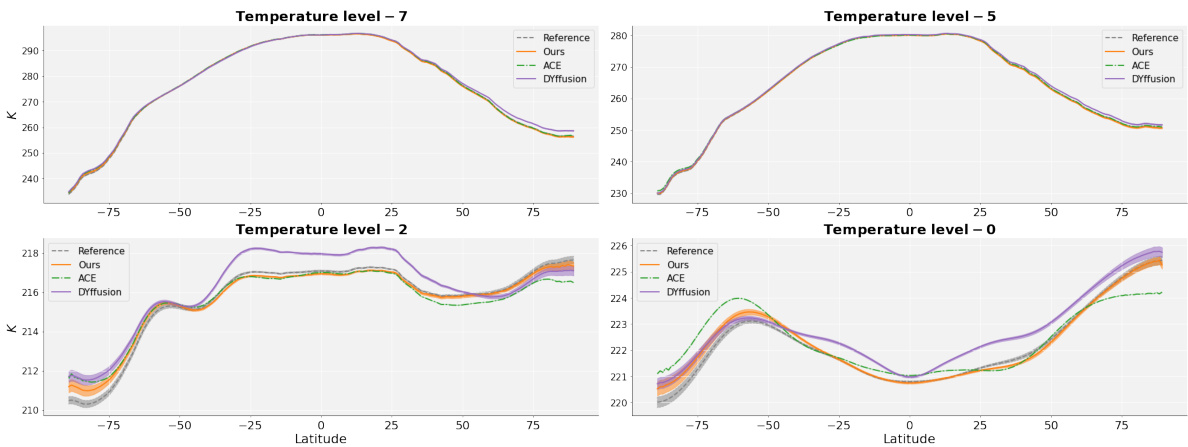
This figure compares zonal means of simulated 10-year time-mean climatologies for four temperature levels (7, 5, 2, 0) across different methods: the proposed method, ACE, and DYffusion, against a reference model. The results show that the proposed model’s zonal means generally align best with the reference model, particularly at lower altitudes. However, all methods demonstrate biases, especially at higher altitudes and near the poles. The biases are more pronounced for DYffusion.
This figure illustrates the discrepancy between a model’s skill in short-term weather forecasting and its long-term climate simulation accuracy. The x-axis represents the average RMSE (Root Mean Square Error) of 5-day weather forecasts, a measure of short-term forecasting skill. The y-axis shows the RMSE of the 10-year time-mean, indicating long-term climate simulation accuracy. Each point represents a distinct model sample or training checkpoint. The scatter plot demonstrates that good short-term weather forecasting skill (low x-axis values) does not guarantee accurate long-term climate simulation (low y-axis values). This highlights the challenge of transferring success in short-term weather forecasting to long-term climate modeling.
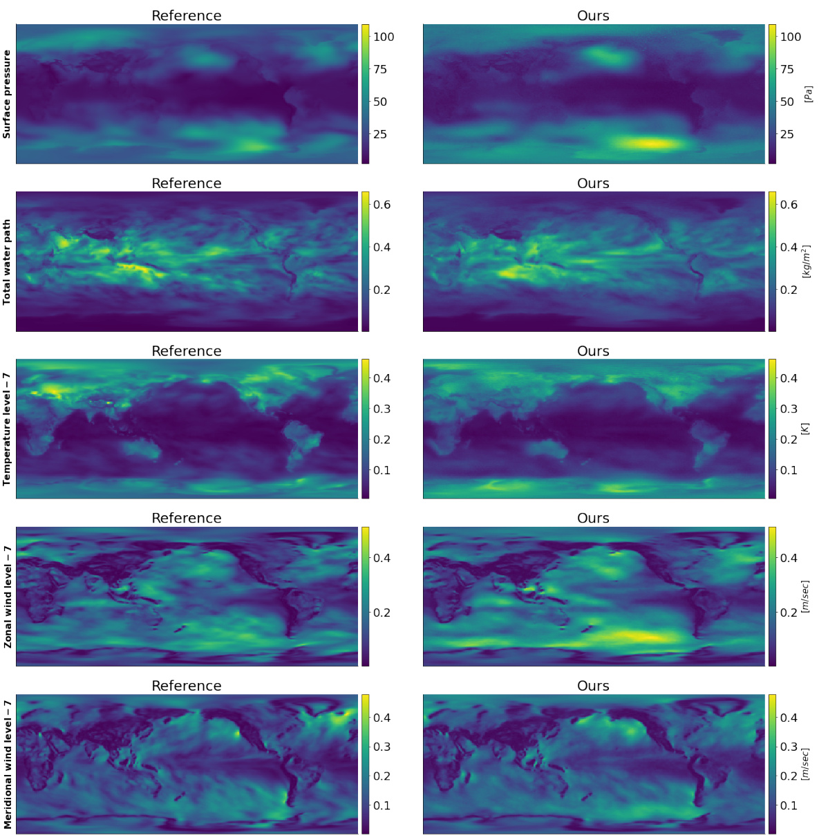
This figure displays global maps visualizing the standard deviation of 10-year time-means for five key climate variables: surface pressure, total water path, near-surface temperature, zonal wind at near-surface level, and meridional wind at near-surface level. Both the reference ensemble and a 25-member ensemble from the proposed Spherical DYffusion model are shown. The maps illustrate that the model’s simulated climate variability closely matches the reference in terms of both spatial patterns and magnitudes. The numerical values are summarized in Table 2.
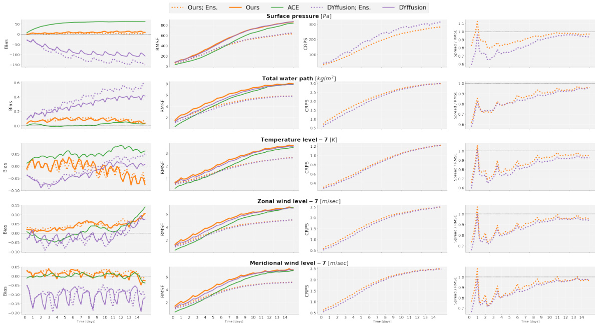
This figure compares the medium-range weather forecasting skill of three different models: Spherical DYffusion, DYffusion, and ACE. For each model, it shows the performance of both a 25-member ensemble and a single forecast. The results highlight that Spherical DYffusion produces competitive probabilistic ensemble weather forecasts. However, it also emphasizes that good ensemble weather forecasting is a necessary, but not sufficient, condition for achieving good climate simulations.

This figure shows the divergence between medium-range weather forecasting skill and long-term climate performance. The x-axis represents the average root mean square error (RMSE) on 5-day weather forecasts, a measure of weather forecasting skill. The y-axis represents the RMSE of the 10-year time-mean, a measure of climate performance. Each point represents a distinct sample or checkpoint epoch from a machine learning model. The lack of correlation highlights that good short-term weather forecasting skill does not guarantee accurate long-term climate simulation.
This figure shows global maps of 10-year time-mean biases for the total water path (TWP) for three different models: the reference model (noise floor), the proposed Spherical DYffusion model, and the ACE baseline model. The maps show the spatial distribution of biases. The accompanying text provides the global mean RMSE and bias values for each model, demonstrating that Spherical DYffusion produces biases very close to the noise floor (i.e., biases explained by inherent climate variability), while ACE shows larger biases indicating systematic model errors.
This figure compares the medium-range weather forecasting skill of three different models: Spherical DYffusion, DYffusion, and ACE. It shows that Spherical DYffusion produces competitive probabilistic ensemble weather forecasts. The figure displays various metrics (RMSE, CRPS, spread-skill ratio) over time (in days) for multiple fields (surface pressure, total water path, temperature, wind speed). While achieving good weather forecasts is necessary, it’s not sufficient for accurate climate simulations, which is a key point highlighted by this figure.
This figure compares the root mean square error (RMSE) of 10-year time-mean predictions for several key climate variables across different models: the proposed Spherical DYffusion model, several baselines (ACE, DYffusion, ACE with stochasticity), and a reference model (FV3GFS). It highlights the superior performance of Spherical DYffusion in reducing climate biases, particularly when using ensemble predictions.
More on tables

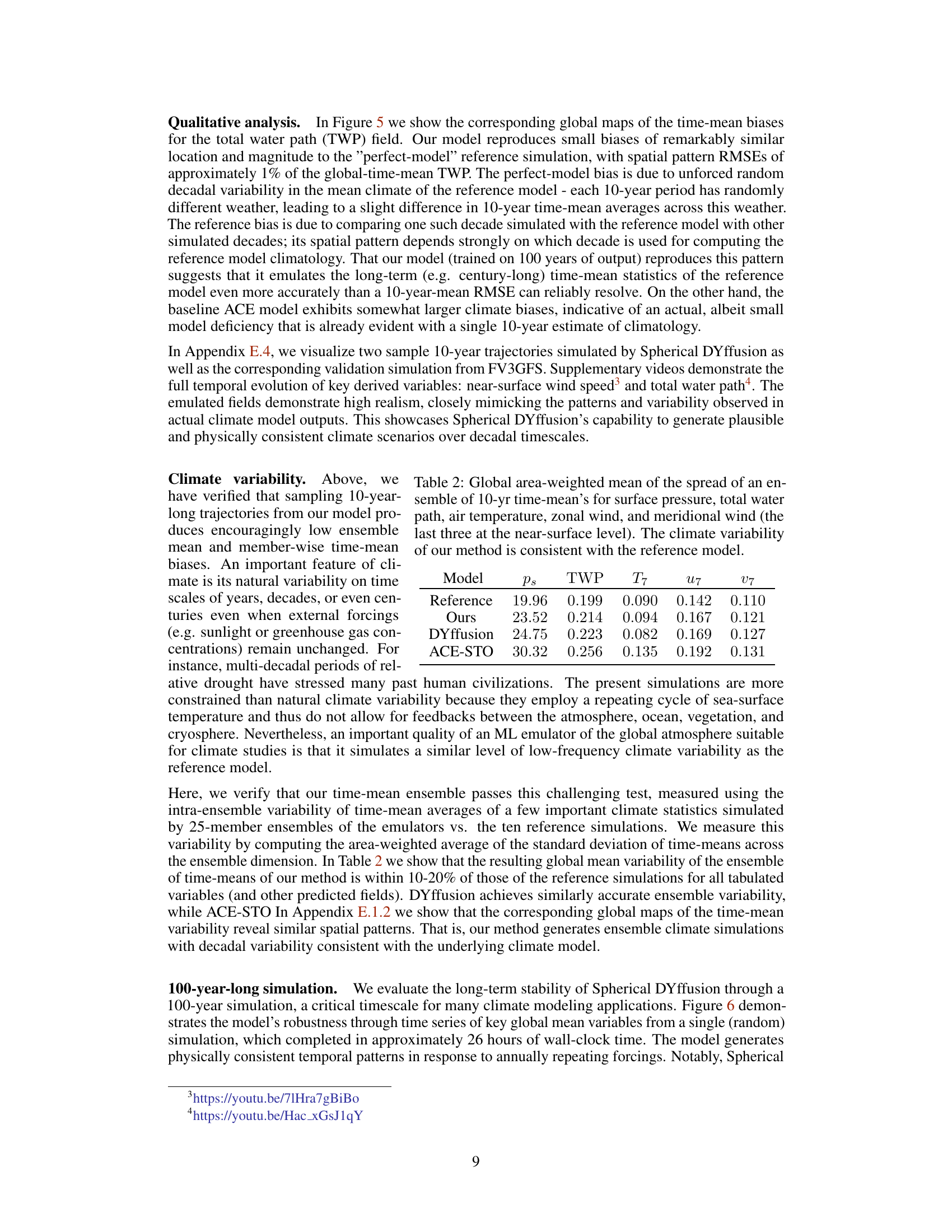
This table presents a comparison of the spread (standard deviation) of 10-year time-mean climate variables across different models. The ‘spread’ represents the variability within each model’s ensemble of simulations. The table shows that the spread generated by the proposed Spherical DYffusion model closely matches the spread observed in the reference FV3GFS model, indicating that the new model accurately captures climate variability. The other models, DYffusion and ACE-STO, show larger spreads than the reference and the proposed model.
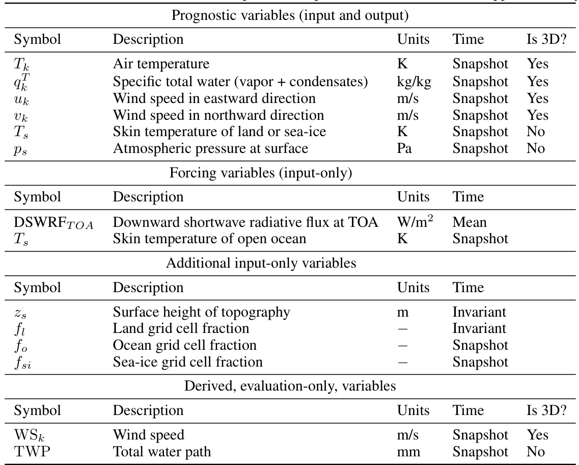
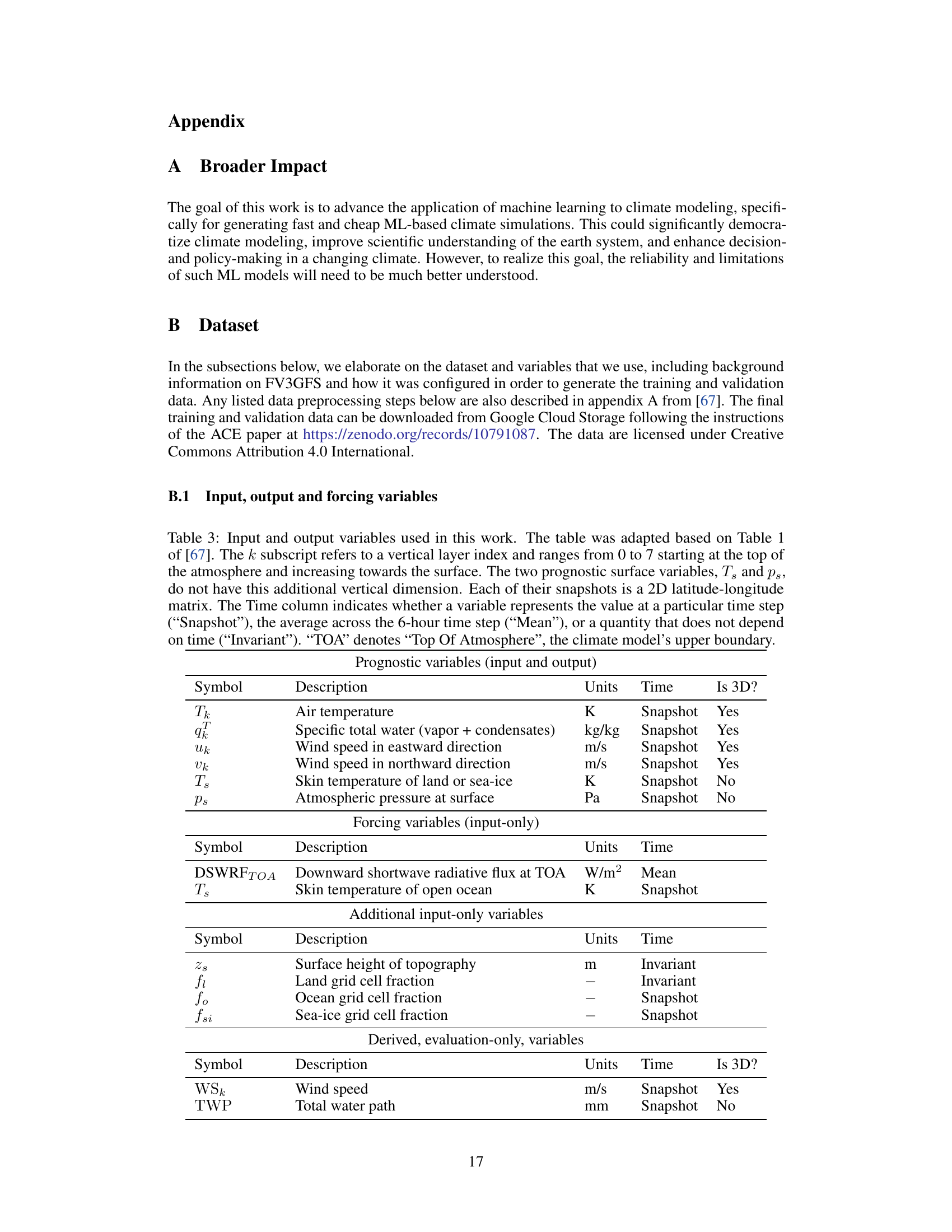
This table lists the input, output, and forcing variables used in the study. It details the description, units, time dependency (snapshot, mean, or invariant), and dimensionality (3D or not) of each variable. The table is organized into sections for prognostic variables (both input and output), forcing variables (input-only), and additional input-only variables. A final section provides a list of derived variables used only for evaluation.
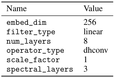
This table shows the hyperparameters used in the SFNO architecture for both the ACE model and the proposed Spherical DYffusion model. It details the values for parameters such as embedding dimension, filter type, number of layers, operator type, scale factor, and number of spectral layers. These settings are critical in determining the performance and characteristics of each model, highlighting the design choices made for optimizing the individual components within each model architecture.
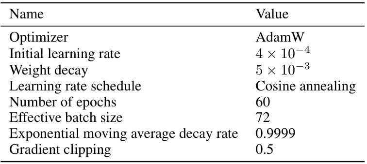
This table presents the hyperparameters used during the optimization process for training the deep learning models. It includes the optimizer used (AdamW), the initial learning rate, weight decay, learning rate schedule (cosine annealing), number of training epochs, effective batch size, exponential moving average decay rate, and gradient clipping value. The effective batch size is dynamically calculated to remain constant across different hardware setups.
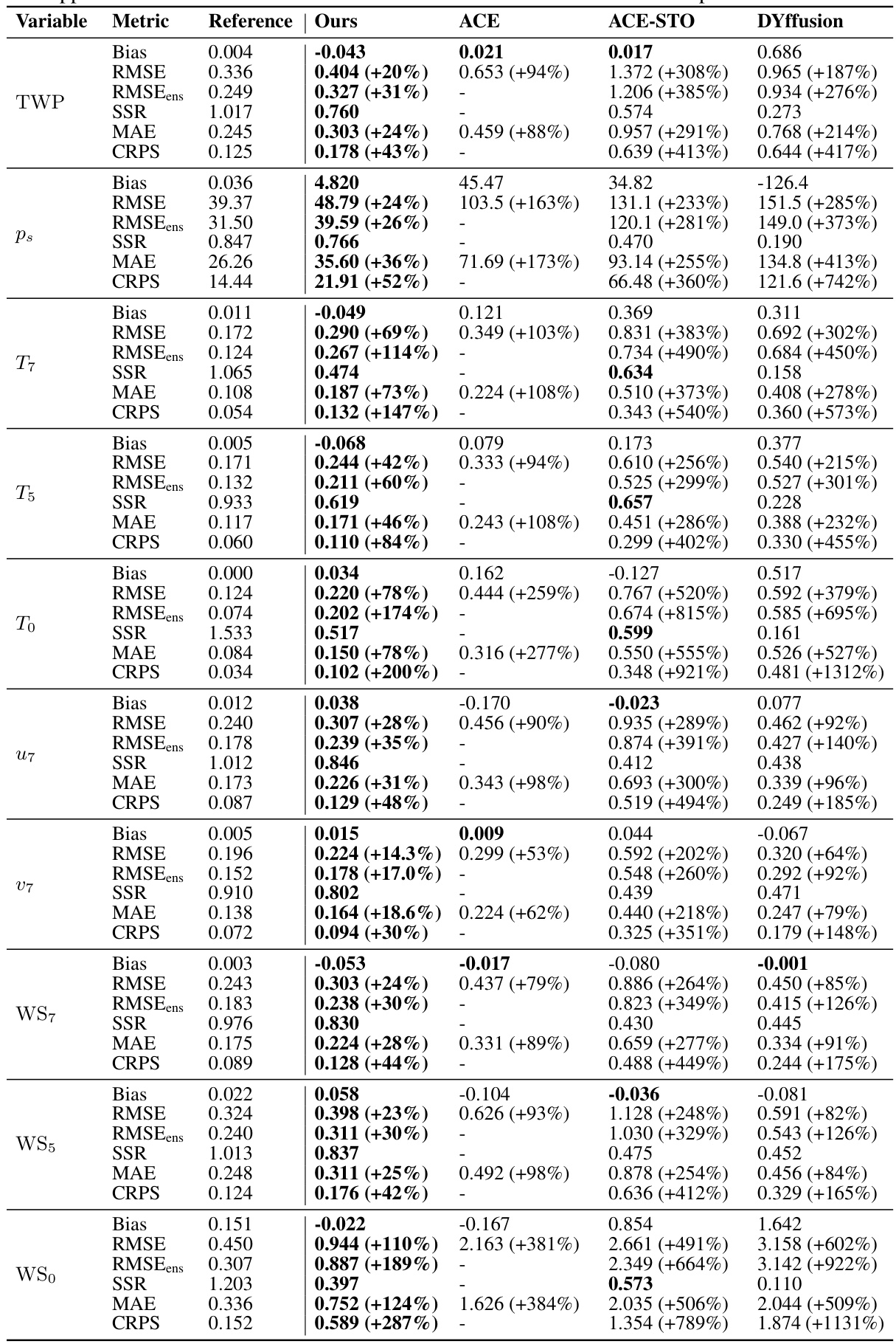
This table presents a comprehensive comparison of different metrics (Bias, RMSE, MAE, RMSEens, SSR, CRPS) for various climate variables (TWP, Ps, T7, T5, To, U7, u7, WS7, WS5, WSo) across four different models: Reference, Ours, ACE, ACE-STO, and DYffusion. It shows the performance of the proposed model (Ours) against the baseline models in terms of bias reduction, accuracy, and uncertainty quantification. The relative changes from the reference model are provided in parentheses to show the improvement or degradation. The table highlights the effectiveness of the proposed method in achieving lower biases and improved accuracy compared to the baselines. Appendix D provides detailed information on the metrics, and Table 3 offers descriptions of the climate variables.
Full paper#
