↗ OpenReview ↗ NeurIPS Proc. ↗ Chat
TL;DR#
Accurately predicting the effects of protein mutations is vital for protein engineering and understanding biological processes. Existing methods often lack reliable uncertainty estimates, hindering their practical use in design and optimization. This makes it challenging to determine which mutations are most promising and trustworthy, especially in a Bayesian Optimization setting where uncertainties are essential to guide the selection of the next mutation to test.
The paper introduces Kermut, a Gaussian Process regression model with a novel composite kernel designed to capture mutation similarities. Kermut demonstrates state-of-the-art performance in predicting the effects of mutations while offering uncertainty estimates. The model’s uncertainty calibration is analyzed, showing reasonable overall calibration but highlighting challenges in instance-specific calibration. Furthermore, Kermut is significantly faster than competing methods, making it a practical tool for researchers in the field.
Key Takeaways#
Why does it matter?#
This paper is crucial for researchers in protein engineering and design. It introduces Kermut, a novel Gaussian process regression model that achieves state-of-the-art accuracy in predicting protein variant effects. Furthermore, Kermut provides reliable uncertainty estimates, which are essential for guiding experimental design and optimization in a Bayesian setting. The work highlights the importance of uncertainty quantification, prompting further research into more robust and accurate prediction methods for protein engineering and design.
Visual Insights#

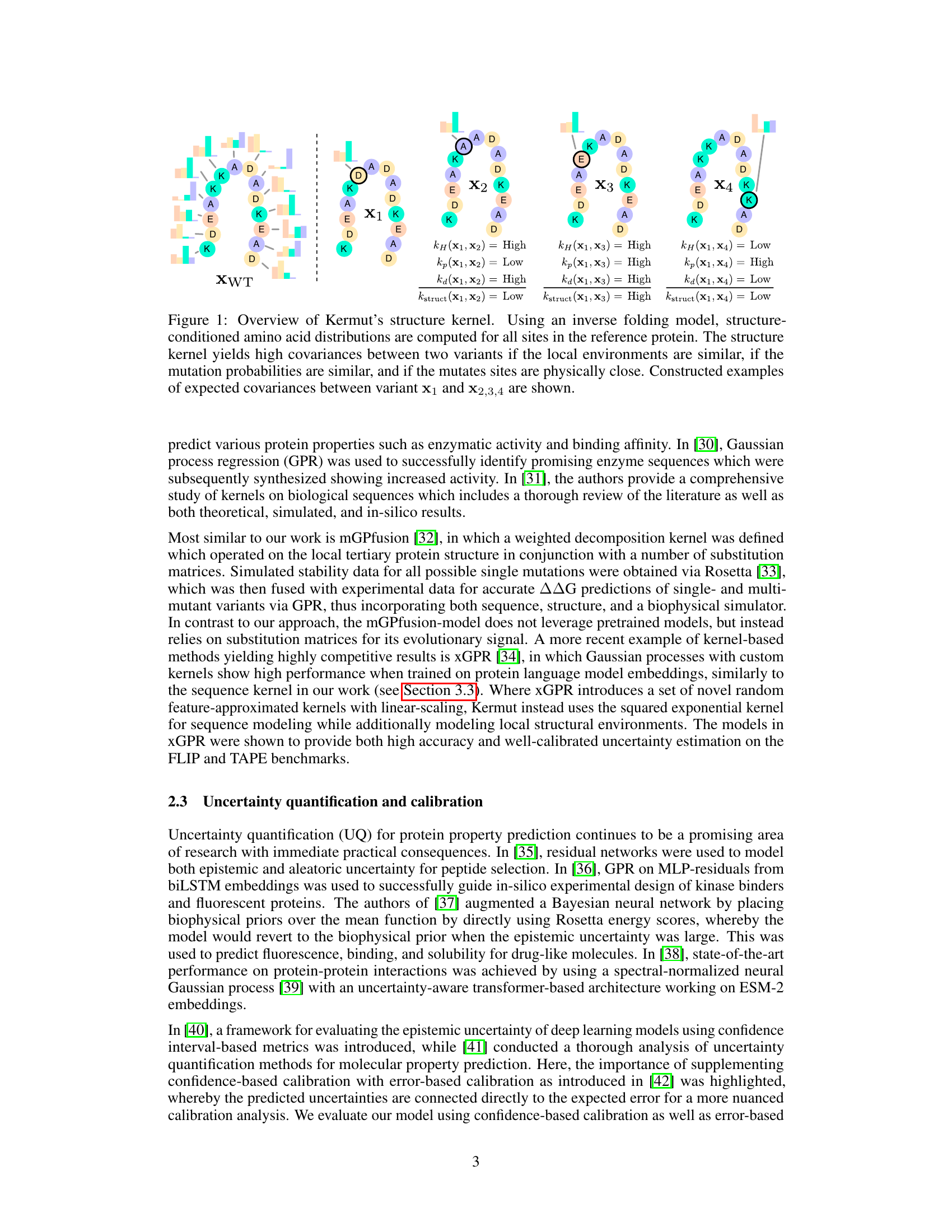
This figure illustrates the structure kernel component of the Kermut model. The model uses an inverse folding model to predict the probability distribution of amino acids at each site in the reference protein, given its structure. The structure kernel then calculates the covariance between pairs of variants based on three factors: 1) The similarity of their local structural environments (assessed using the Hellinger distance between amino acid distributions), 2) the similarity of their mutation probabilities, and 3) the physical proximity of the mutated sites. The figure shows four example variants (x1-x4), each compared against a reference protein (xWT), highlighting how the kernel would compute high or low covariances based on these three factors.
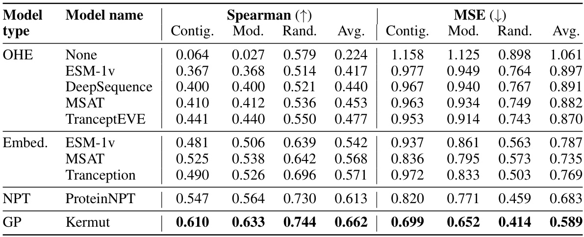
This table shows the performance of the Kermut model and other state-of-the-art models on the ProteinGym benchmark. The benchmark includes three different cross-validation schemes: random, modulo, and contiguous. The table reports the Spearman correlation and Mean Squared Error (MSE) for each model and scheme. The ‘Contig.’, ‘Mod.’, and ‘Rand.’ columns refer to contiguous, modulo, and random split schemes, respectively. ‘OHE’ and ‘NPT’ represent one-hot encoding and non-parametric transformer model types, respectively. Bold values indicate the best performance for each metric.
In-depth insights#
Composite Kernel#
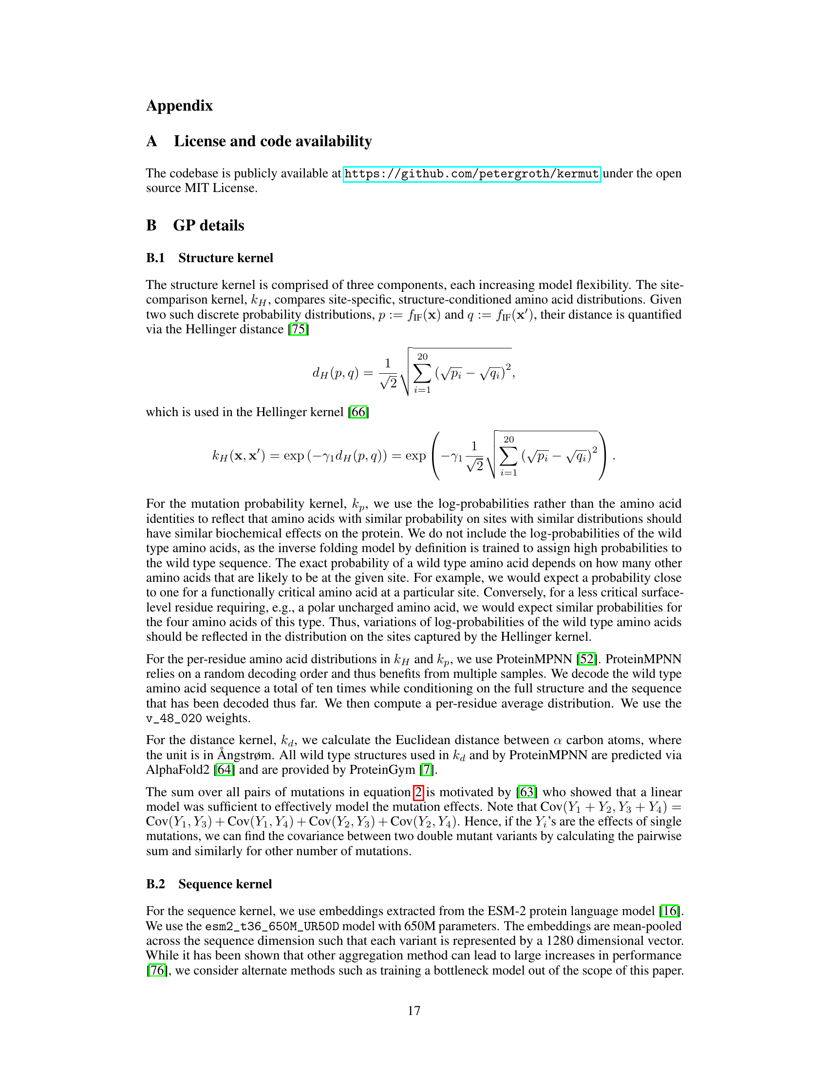
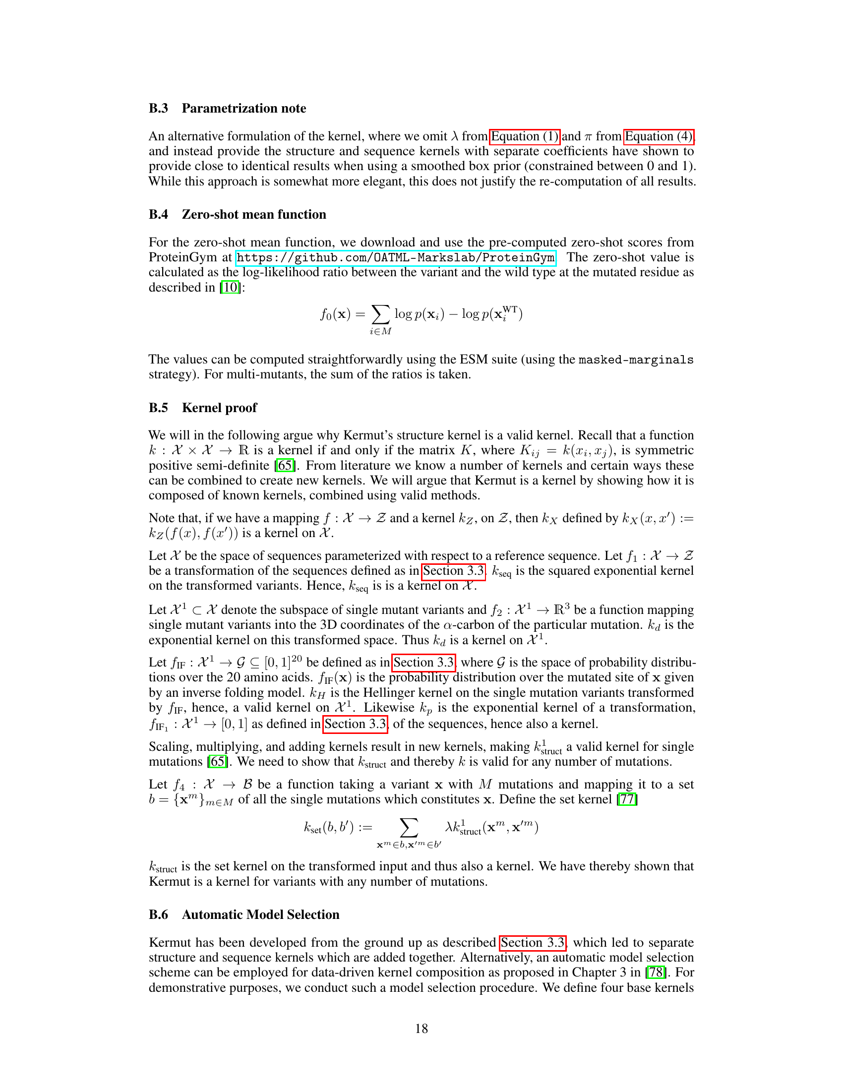
The heading ‘Composite Kernel’ strongly suggests a machine learning approach leveraging the power of combining multiple kernel functions. This composite design likely aims to capture diverse aspects of protein variant effects, integrating information from different sources such as sequence similarity (using existing protein language models), structural features (e.g., spatial proximity of residues), and potentially even biophysical properties. By combining kernels, the model can address limitations of individual kernels, such as the inability of sequence-based kernels to fully capture structural context. The weighting scheme used to combine the kernels is crucial; it needs to balance contributions, preventing a single kernel from dominating the prediction. This composite kernel approach is particularly relevant in the context of protein variant effect prediction, which involves complex interactions. The effectiveness of the approach depends on the careful selection and combination of constituent kernels, as well as the optimization of hyperparameters governing the weighting scheme. Ultimately, the success of a composite kernel hinges on achieving superior prediction accuracy compared to individual kernels, possibly alongside improved uncertainty quantification.
Uncertainty Quant#
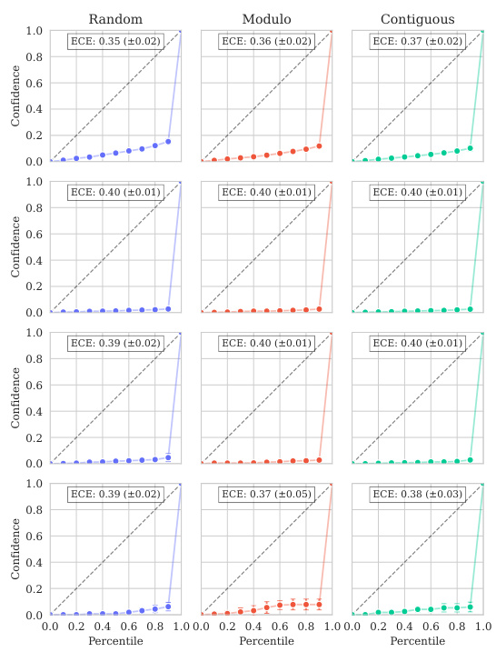
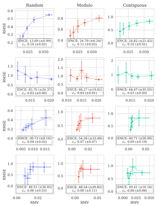
Uncertainty quantification in protein variant effect prediction is crucial for reliable application of predictive models in protein engineering and design. Accurate uncertainty estimates are essential for guiding experimental efforts, informing the selection of promising variants, and providing a measure of confidence in predictions. The paper investigates uncertainty quantification using a Gaussian Process (GP) model, highlighting the challenges in achieving well-calibrated uncertainty, particularly at the instance-specific level. While overall model calibration might be satisfactory, instance-specific calibration remains a significant challenge. This underscores the need for further research to improve methods for uncertainty estimation in this domain and emphasizes the importance of reporting and analyzing uncertainty metrics in protein variant effect prediction studies. Future work could explore more sophisticated kernel designs or alternative model architectures to improve uncertainty calibration. A key takeaway is the importance of moving beyond simple calibration metrics towards more nuanced assessments of uncertainty reliability, ensuring that uncertainty estimates are truly informative and reliable for practical decision making.
ProteinGym Bench#
The ProteinGym benchmark is a comprehensive suite of datasets designed for evaluating the performance of protein variant effect prediction methods. Its strength lies in its standardized datasets, covering various aspects like substitutions, insertions, and deletions, and encompassing various traits. This diversity allows for a rigorous assessment of different model architectures and strategies. The benchmark’s focus on uncertainty quantification is a significant advancement, promoting a more reliable and practical application of these predictive models in the field of protein engineering. This includes instance-to-instance uncertainty estimates, a crucial element for guiding experimental efforts efficiently. The availability of multiple cross-validation schemes, including random, modulo, and contiguous, further enhances the robustness and generalizability of model evaluations.
Ablation Study#
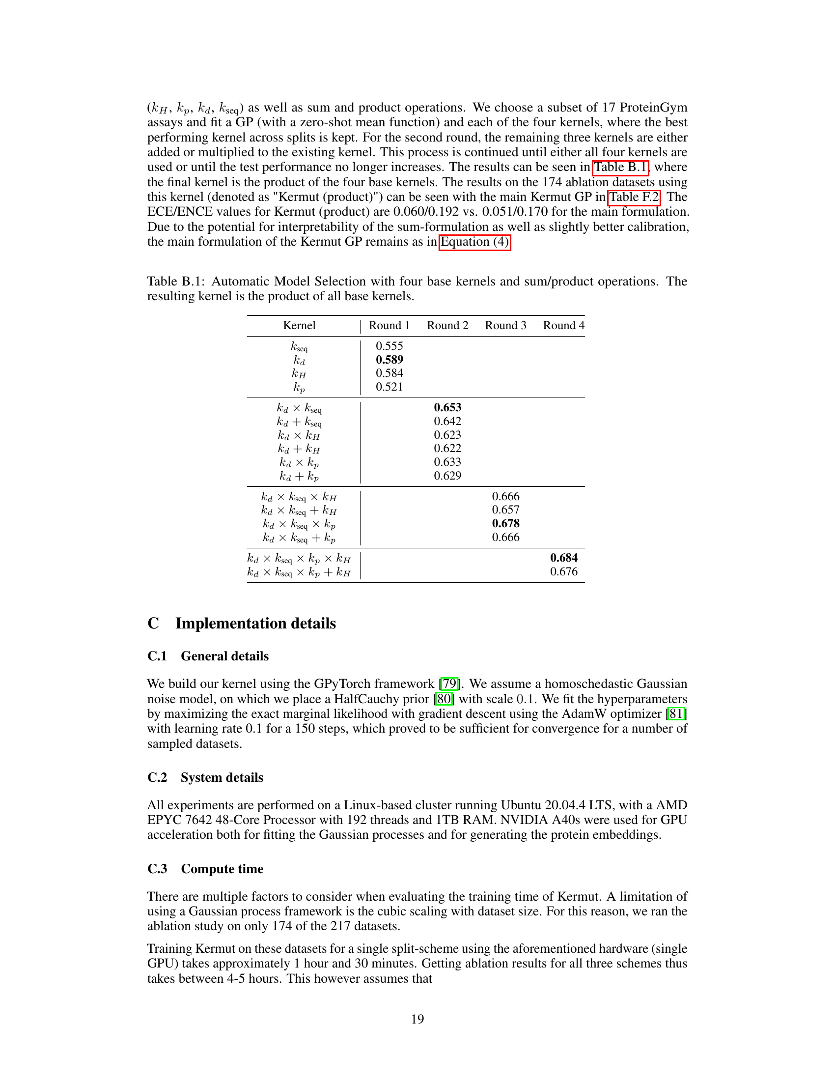
An ablation study systematically removes or alters components of a model to assess their individual contributions. In the context of the provided research, an ablation study on the composite kernel would involve successively removing kernel components (e.g., the structure kernel, sequence kernel, or specific sub-components within the structure kernel) to observe their individual impact on the model’s overall performance, such as Spearman correlation and MSE. The results would quantify the relative importance of each component in achieving state-of-the-art results. A well-designed ablation study provides valuable insights into the model’s architecture, highlighting which components are crucial and which are less impactful. It could reveal synergistic effects between components or potential redundancy. Furthermore, ablation studies help determine the necessity of each component in achieving the model’s performance, potentially guiding future model improvements by focusing development on the most critical aspects. The ablation results, therefore, demonstrate the model’s robustness and the contribution of each component, providing crucial information for understanding and improving the model’s design and calibration
Future Work#
Future work could explore several promising avenues. Improving uncertainty calibration, particularly at the instance level, is crucial. This might involve investigating more sophisticated kernel designs or incorporating additional data sources. Another key area is extending Kermut to handle insertions and deletions. This requires moving beyond the single-site mutation focus and developing a model that can effectively represent more complex sequence variations. Scaling Kermut to larger datasets is essential for wider applicability, potentially through the use of approximate inference methods or by leveraging parallel computing techniques. Lastly, exploring different zero-shot methods and their impact on uncertainty quantification should be studied, and more advanced hyperparameter optimization techniques should be investigated. Addressing epistatic effects more directly in the model would likely improve accuracy and uncertainty quantification on datasets exhibiting strong epistasis, requiring more complex kernel designs and perhaps even moving beyond GP models.
More visual insights#
More on figures

This figure shows the distribution of predictive variances from the model for datasets containing double mutations. It breaks down the variance based on different training and testing scenarios (domains). The first three represent standard ProteinGym split schemes (random, modulo, contiguous). The next two show training on both single and double mutants then testing on single mutants and double mutants separately. The final domain shows the challenging extrapolation scenario of training only on single mutants but testing on double mutants.
This figure illustrates the structure kernel of Kermut. The kernel uses an inverse folding model to compute structure-conditioned amino acid distributions for each site in the reference protein. It then calculates the covariance between two variants based on the similarity of their local environments, the similarity of their mutation probabilities, and their physical distance. The figure shows example covariances between variant x₁ and variants x₂, x₃, x₄, illustrating how the kernel captures relationships between mutations based on structural context and mutation similarity.
This figure illustrates the structure kernel used in the Kermut model. It shows how the kernel considers three factors when assessing the similarity between two protein variants: (1) The similarity of the local structural environments of the mutated sites, (2) the similarity of the mutation probabilities at those sites (as predicted by an inverse folding model), and (3) the physical distance between the mutated sites. The examples provided show how the kernel generates higher covariances for variants with similar local environments and mutation probabilities, and that are physically close together.
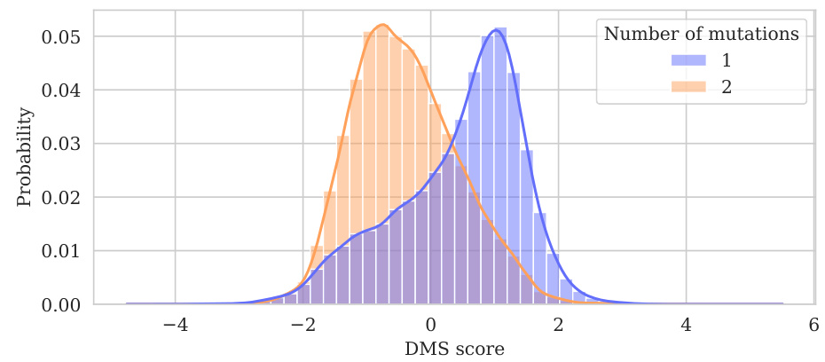
This figure shows the distribution of normalized assay values for datasets containing multiple mutations. Data from 51 datasets (out of 69 with multiple mutations, excluding one dataset with excessively many mutations) are shown, with each dataset containing fewer than 7500 variants. The histograms are separated by the number of mutations in each variant (1 or 2 mutations). The figure illustrates how the distribution of assay values varies depending on the number of mutations, with double mutations tending to correlate with lower fitness.
This figure shows the distribution of predictive variances for datasets containing double mutants. The x-axis represents different domains categorized by the type of mutation testing and training data used: single-mutant training and testing, training on both single and double mutants and testing on both, and extrapolation where training used only single mutants while testing used double mutants. The y-axis shows the predictive variance, a measure of uncertainty in the model’s predictions. Each boxplot summarizes the distribution of predictive variances across multiple datasets within each domain, allowing for a visual comparison of uncertainty levels across different prediction scenarios.
This figure shows the distribution of predictive variances for datasets that include double mutants, categorized by the type of mutation domain. The three initial columns show the distributions for the three ProteinGym cross-validation schemes (random, modulo, contiguous). The fourth and fifth columns compare the distributions when training occurs on both single and double mutants, with testing on only single, and only double mutants respectively. The final column shows the distribution of predictive variances when training only occurs on single mutants while testing is performed on double mutants, representing an extrapolation domain.
This figure shows the distribution of predictive variances for datasets that include double mutants. The x-axis represents the different domains used for training and testing the model, while the y-axis represents the predictive variance. The three first domains correspond to the three split schemes of the ProteinGym benchmark (random, modulo, contiguous), while the other three domains show the predictive variance when training and testing on both single and double mutants, and extrapolating from single mutants to double mutants. This shows that when the training data is closer to the test data, the uncertainties are smaller. This is reflected in the low uncertainty in the first three domains where only single mutants are used.
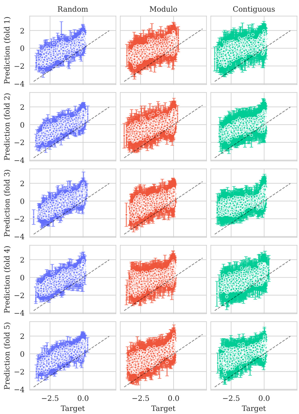
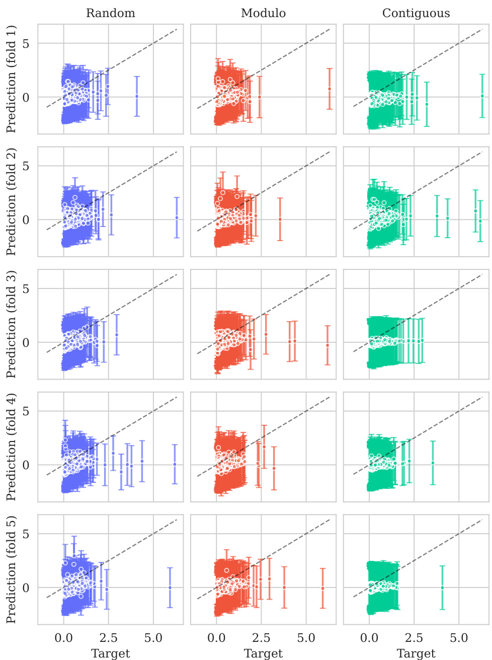
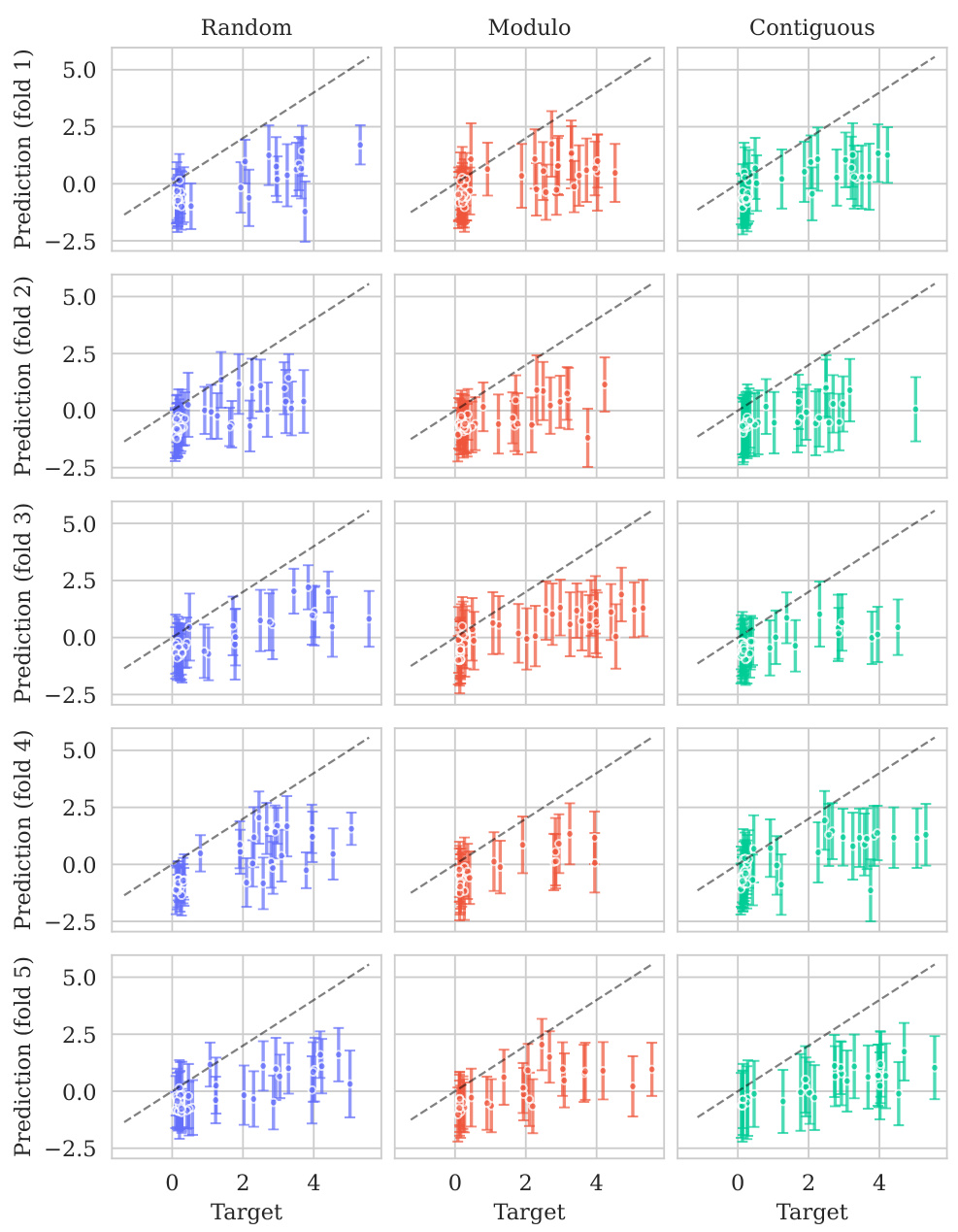
This figure displays the predicted values plotted against the true values for the BLAT_ECOLX_Stiffler_2015 dataset. The plot is separated into columns representing different cross-validation schemes (Random, Modulo, Contiguous) and rows showing the results for each test fold (five folds total). The dashed diagonal line indicates a perfect prediction; points closer to this line show better predictive accuracy. The error bars represent ±2 standard deviations, providing a visual representation of model uncertainty. The distribution and spread of points around the diagonal line visually illustrate the calibration of the model’s uncertainty estimates for this specific dataset across various splitting schemes.
This figure shows the distribution of predictive variances for datasets containing double mutants. It compares the variance across six different scenarios (domains) which vary how the model is trained (single vs. double mutants) and tested (single vs. double mutants). The first three domains represent standard ProteinGym split schemes. The final domain represents an extrapolation setting.
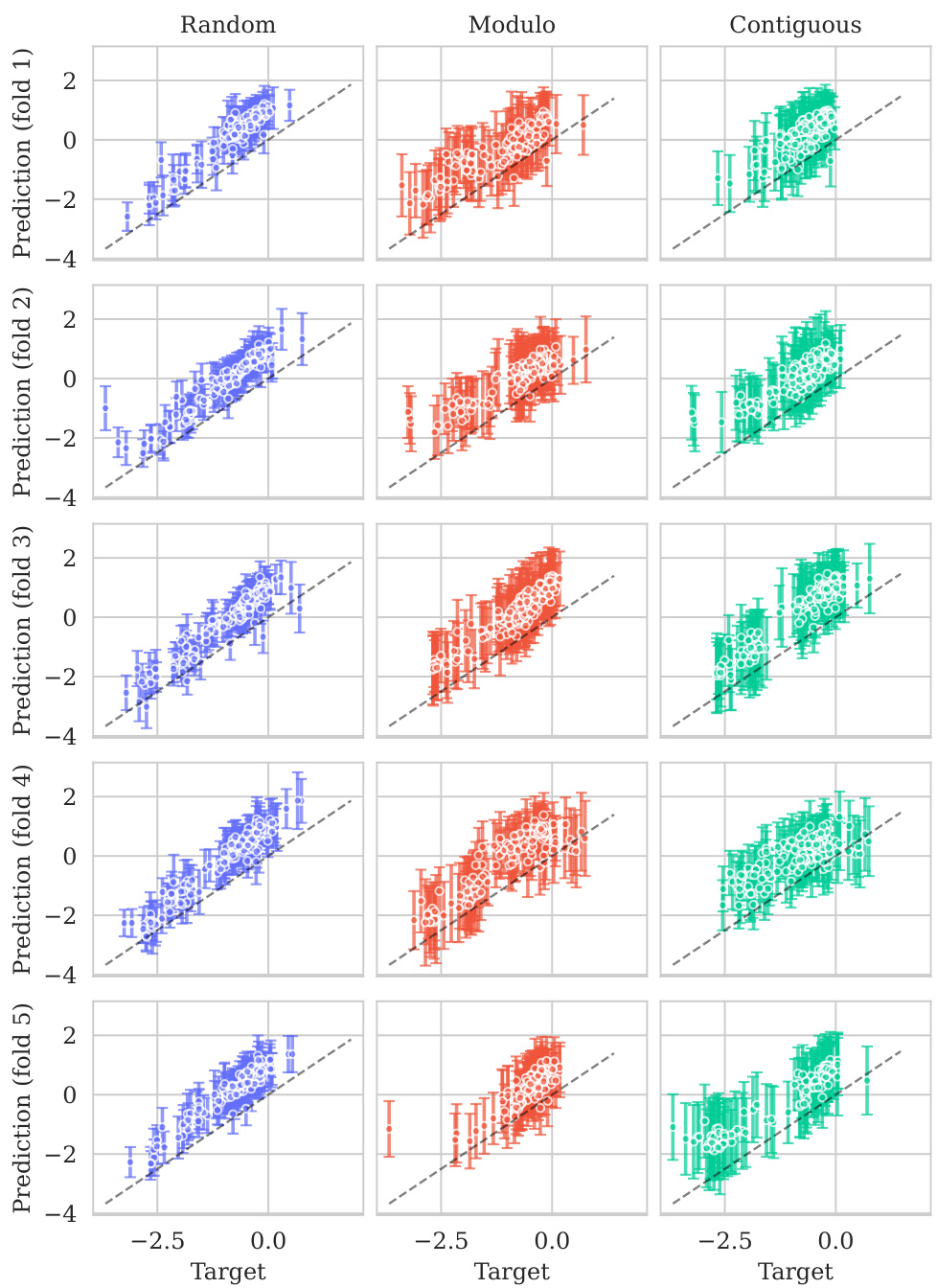
This figure shows the predicted means with their uncertainty intervals (2σ) plotted against their true values for the BLAT_ECOLX_Stiffler_2015 dataset. It compares the model’s predictions across five different cross-validation folds (rows) and three different schemes (columns: random, modulo, and contiguous). The dashed diagonal line represents perfect prediction. The extent to which the points deviate from this line indicates the accuracy of the model’s predictions.
This figure shows the distribution of predictive variances for datasets containing double mutants. The x-axis represents the predictive variance, and the y-axis shows the different domains. The first three domains represent the three split schemes from the ProteinGym benchmark, which are examples of interpolation. The fourth and fifth domains show the distributions when training on both single and double mutants and testing separately on each. The last domain shows the distribution when training only on single mutants but testing on double mutants (extrapolation). The figure demonstrates how uncertainties vary across different mutation domains and experimental settings.
The figure shows the distribution of predictive variances in six different mutation domains. The first three domains are the standard ProteinGym splits (random, modulo, contiguous). The next two domains train on both single and double mutations then test on single or double mutations, respectively. The final domain trains on single mutations only then tests on double mutations.
This figure illustrates the structure kernel of Kermut, a Gaussian process regression model for predicting protein variant effects. The kernel leverages signals from pretrained sequence and structure models to capture mutation similarity. The structure kernel uses an inverse folding model to predict amino acid distributions at various sites in the protein, conditioned on the local structural environments. The figure demonstrates that the kernel assigns high covariances between pairs of variants with similar local environments, similar mutation probabilities, and close physical proximity of the mutated sites. Examples of covariance between a reference variant and three other variants are visually presented.
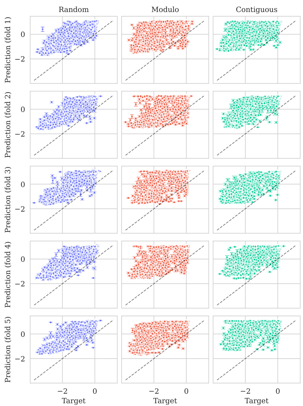
This figure displays the predicted versus true values for the BLAT_ECOLX_Stiffler_2015 dataset. The x-axis represents the true values and the y-axis represents the predicted means, with error bars indicating ±2 standard deviations. The data is broken down by five cross-validation folds (rows) and three schemes (columns: Random, Modulo, Contiguous). The dashed diagonal line shows the ideal prediction where predicted values perfectly match true values. Deviations from this line illustrate the model’s predictive accuracy for each fold and scheme.
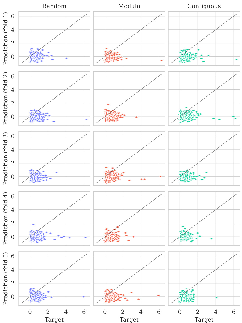
This figure displays the predicted means with error bars (±2σ) plotted against the true values for the BLAT_ECOLX_Stiffler_2015 dataset. It’s a visual representation of the model’s performance across five different cross-validation folds (rows) and three different splitting schemes: random, modulo, and contiguous (columns). The dashed diagonal line represents perfect prediction; deviations from this line indicate prediction errors. The error bars show the uncertainty associated with each prediction.
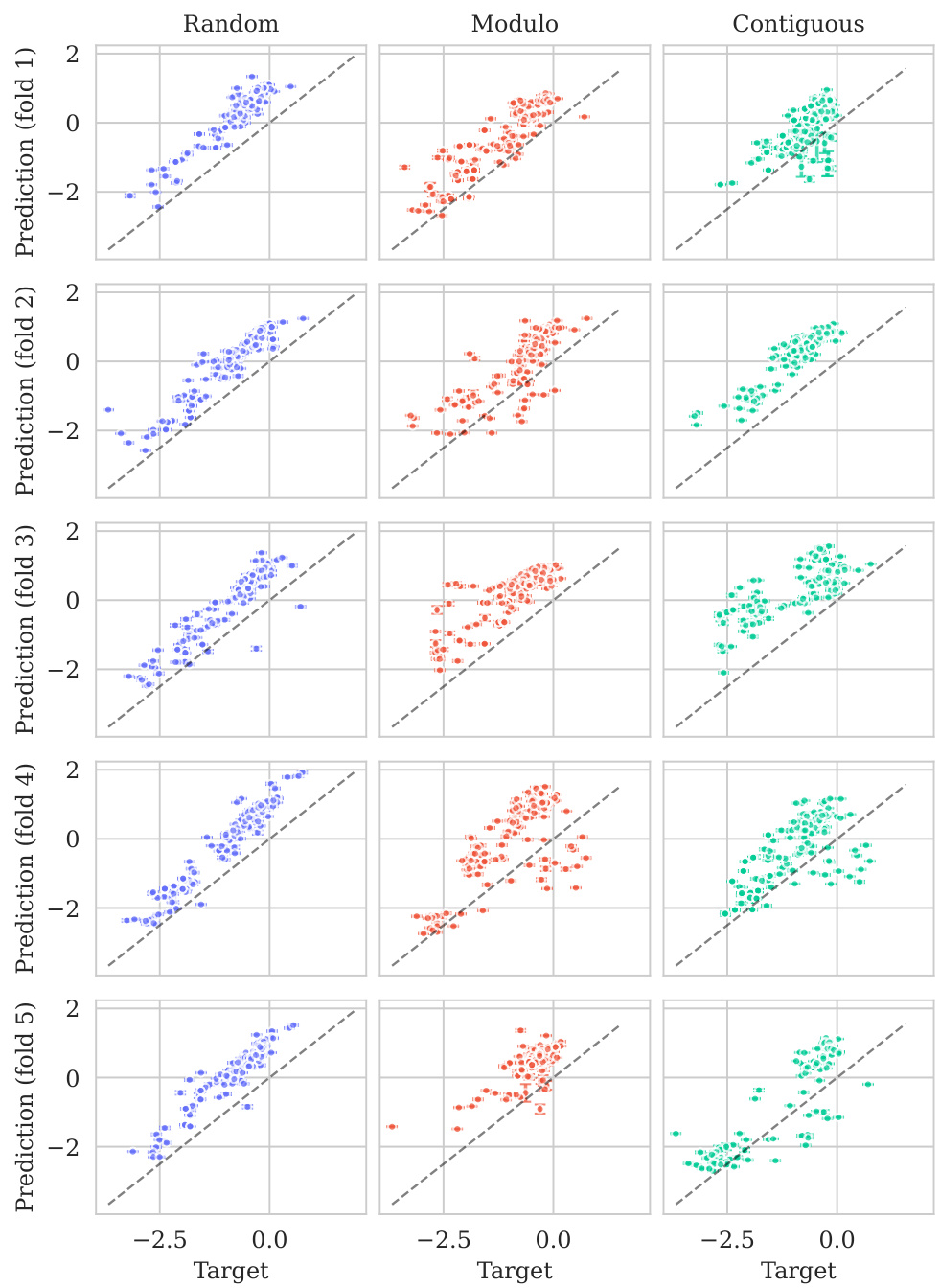
This figure displays the predicted means with their uncertainty intervals (±2σ) plotted against the true values for the BLAT_ECOLX_Stiffler_2015 dataset. It shows the model’s performance across five different test folds and three cross-validation schemes (Random, Modulo, Contiguous). The dashed diagonal line represents perfect prediction, where the predicted and true values would align. Deviations from this line indicate prediction errors. This visualization helps assess the model’s calibration (how well the predicted uncertainty reflects the actual error) and overall prediction accuracy for this specific dataset.
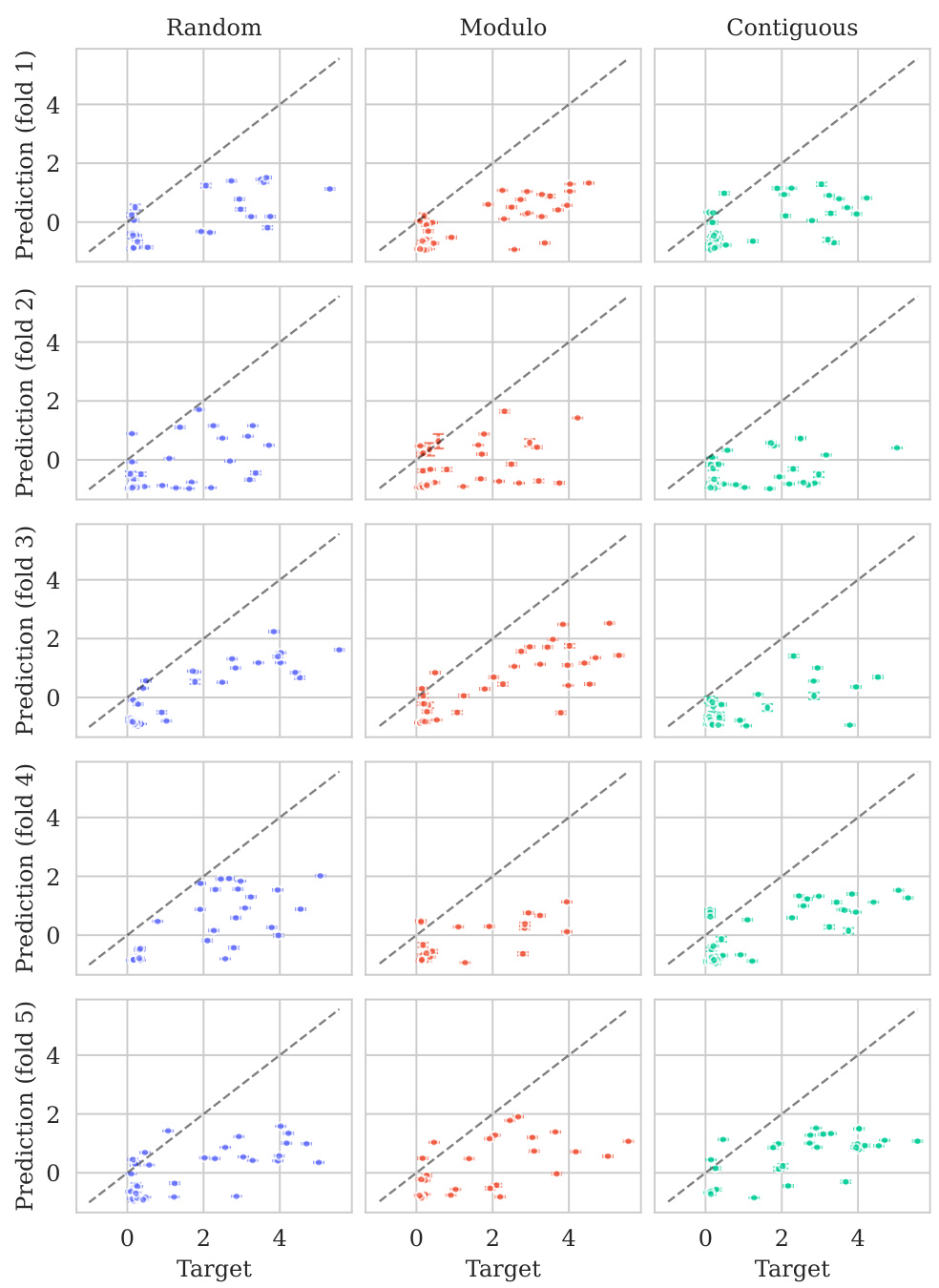
This figure displays the predicted versus true values for the BLAT_ECOLX_Stiffler_2015 dataset. It shows the results of five-fold cross-validation, with each row representing a different test fold and each column representing a different cross-validation scheme (Random, Modulo, Contiguous). The dashed diagonal line represents perfect prediction. The error bars represent the ±2σ confidence intervals of the predictions.
This figure illustrates how Kermut’s structure kernel works. The kernel uses an inverse folding model to predict the probability distributions of amino acids at each site in the protein, given the protein’s structure. The model determines the covariance between two protein variants based on three factors: the similarity of their local structural environments, the similarity of their mutation probabilities, and the physical distance between the mutated sites. The examples in the figure show how these factors combine to produce the covariance.
This figure illustrates the structure kernel used in the Kermut model. The kernel leverages information from inverse folding models to capture relationships between the amino acid distributions at different sites in a protein. High covariances are observed between pairs of mutations where local environments are similar, mutation probabilities are similar, and the sites are physically close together. The example shown highlights this concept using four variant sites (x1, x2, x3, x4).
This figure illustrates how Kermut’s structure kernel works. It uses an inverse folding model to predict amino acid distributions at each site in a protein, given the protein’s structure. The kernel then compares these distributions to assess similarity between two protein variants. The figure shows that the kernel gives high covariance (similarity) between variants when the local environments of the mutated sites are similar, when the probabilities of the mutations are similar, and when the mutated sites are physically close together. Three example pairs of variants are given to show how covariances are determined.
This figure illustrates the structure kernel of Kermut, a Gaussian process regression model. The kernel leverages signals from pretrained sequence and structure models to model mutation similarity. The illustration shows how the structure kernel computes covariances between different variants by considering the similarity of their local structural environments, mutation probabilities, and physical distances between mutated sites. The examples provided visually depict how the kernel would produce high or low covariances depending on these three factors.
This figure illustrates the structure kernel of Kermut, a Gaussian process regression model for protein variant effect prediction. The structure kernel leverages information from pretrained sequence and structure models to capture the effects of mutations. It combines signals from three sources: 1) the Hellinger kernel (kh) measures the similarity of amino acid distributions at different sites, conditioned on their local structure; 2) the mutation probability kernel (kp) assesses how likely a specific mutation is at a given site; 3) the Euclidean distance kernel (kd) considers the physical proximity of mutated sites. The figure depicts example covariances showing that the kernel assigns high covariances between variants if their local environments are similar, if the mutation probabilities are similar, and if the mutated sites are physically close.
This figure illustrates the structure kernel of the Kermut model. The structure kernel leverages an inverse folding model to compute structure-conditioned amino acid distributions for all sites in a reference protein. The kernel calculates high covariances between two variants if their local structural environments are similar, their mutation probabilities are similar, and the mutated sites are physically close. The figure includes schematic examples showing how the kernel evaluates covariances between different variant pairs.
This figure illustrates the structure kernel of Kermut, which models mutation similarity based on the local structural environments of mutated sites. It uses an inverse folding model to predict amino acid distributions for each site, conditioned on its local environment. The kernel assigns high covariances between two variants if their local environments, mutation probabilities, and the distances between mutated sites are similar. Three example pairs of variants (x₁ with x₂, x₃, x₄) are shown to illustrate different levels of covariance (high or low) based on these factors.
This figure illustrates the structure kernel of the Kermut model, which is a crucial component for capturing mutation similarity based on the local structural environment of residues in a protein. It uses an inverse folding model to calculate structure-conditioned amino acid distributions for each site. The kernel assigns high covariances between two variants if their local environments are similar, their mutation probabilities are similar, and the mutated sites are physically close. The examples shown depict the expected covariances between a reference variant and three other variants, illustrating how the kernel assesses similarity based on these three factors.
More on tables

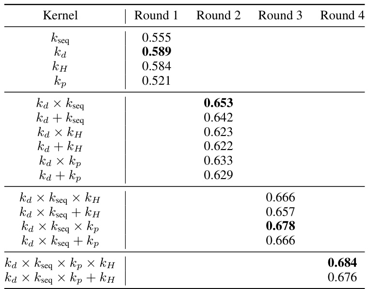
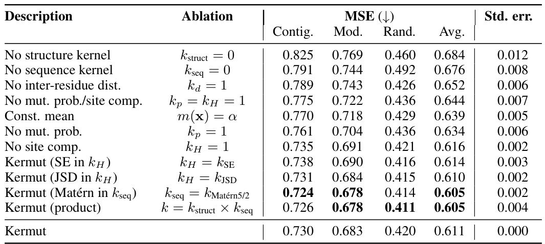
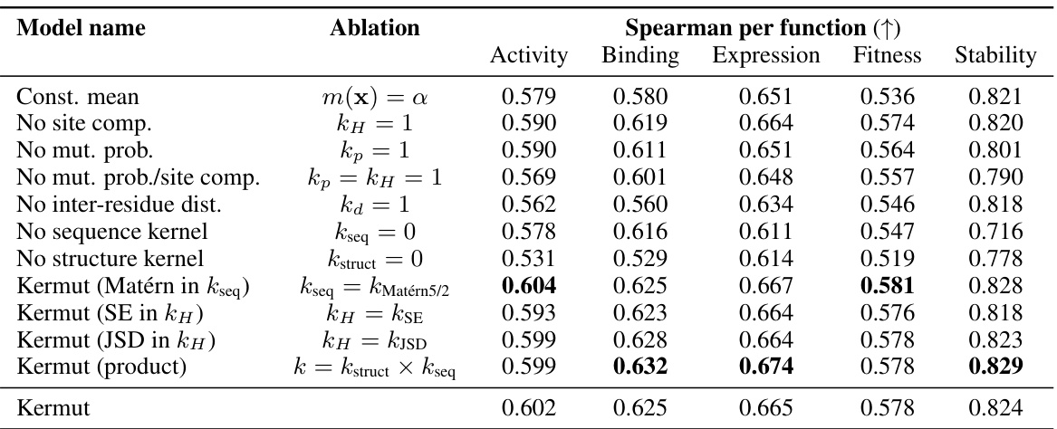
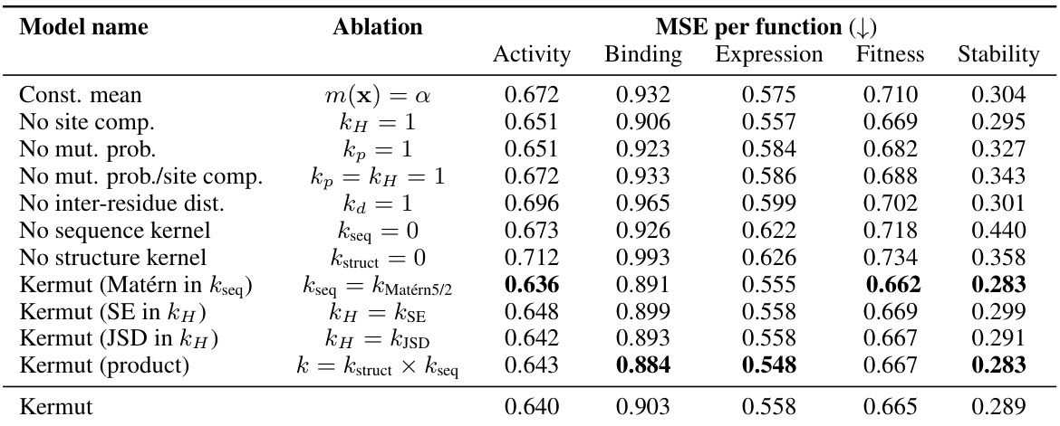
This table presents the results of an ablation study conducted on the Kermut model. Key components of the composite kernel were systematically removed or altered, and the resulting impact on the model’s performance, measured using Spearman correlation, was evaluated on a subset of assays from the ProteinGym benchmark. The table shows the changes in performance relative to the full Kermut model for each ablation, allowing for a quantitative assessment of the contribution of each kernel component to the overall model performance.

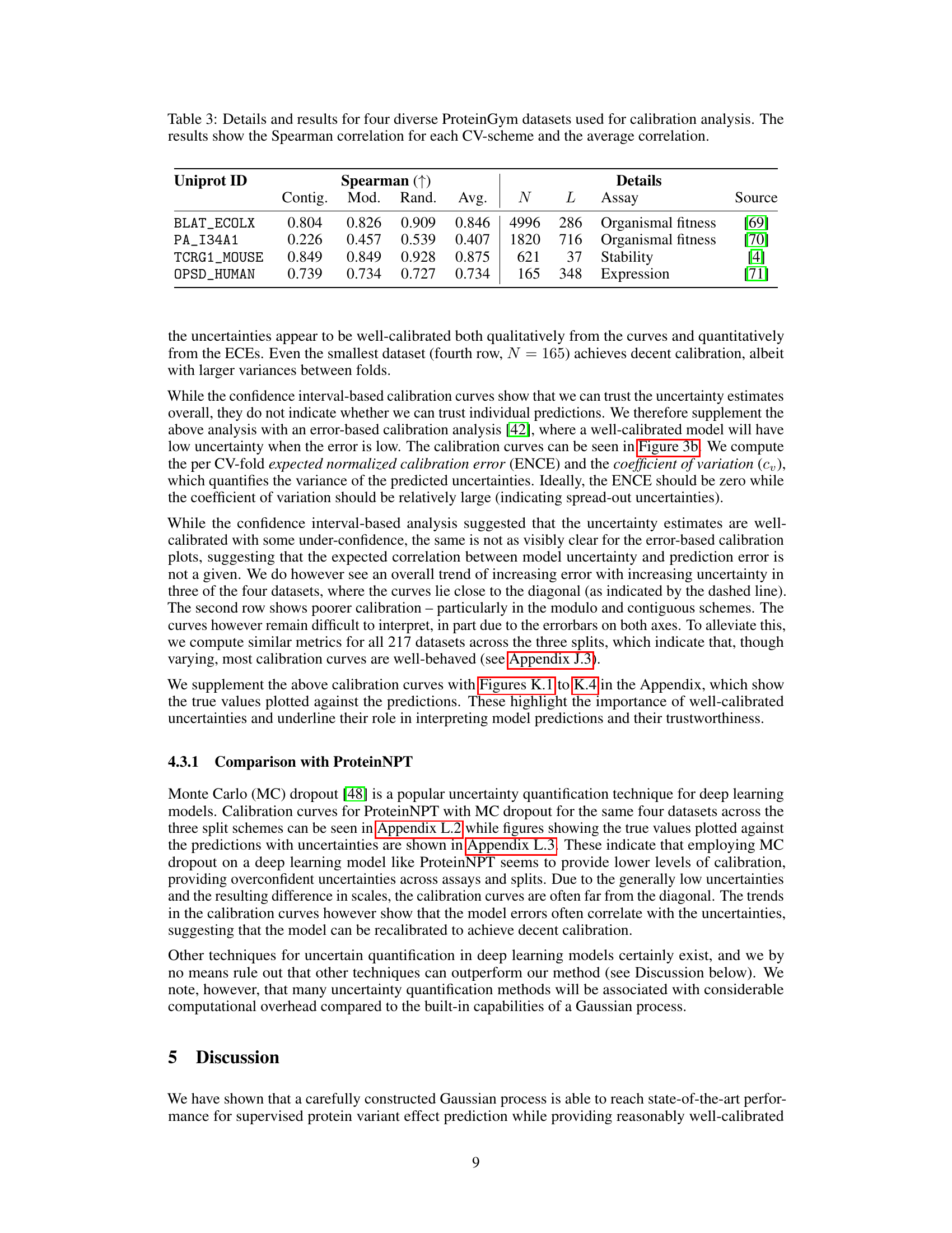
This table presents the results of the Kermut model and other state-of-the-art models on the ProteinGym benchmark. The benchmark evaluates protein variant effect prediction using three different cross-validation schemes: contiguous, modulo, and random. The table shows the Spearman correlation and Mean Squared Error (MSE) for each model and scheme, with the best results for each metric bolded. The model types (OHE and NPT) refer to the input representation used: one-hot encoding and non-parametric transformers, respectively. The table highlights Kermut’s superior performance across all schemes, particularly in the more challenging contiguous and modulo settings.
This table presents the performance of the Kermut model and several other models on the ProteinGym benchmark, which evaluates protein variant effect prediction. The benchmark includes three cross-validation schemes: contiguous, modulo, and random. The table shows Spearman correlation and Mean Squared Error (MSE) for each model across these schemes. Kermut’s performance is highlighted in bold, demonstrating its superiority, especially in the more challenging modulo and contiguous settings.

This table presents the performance of Kermut and other state-of-the-art methods on the ProteinGym benchmark. The benchmark includes three different cross-validation schemes, and the table shows the Spearman correlation and Mean Squared Error (MSE) for each method across the schemes. Kermut demonstrates superior performance across all schemes, with significant improvement in the challenging modulo and contiguous settings.
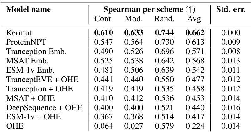
This table presents the performance of Kermut and other state-of-the-art methods on the ProteinGym benchmark for protein variant effect prediction. The benchmark includes three different cross-validation schemes: contiguous, modulo, and random. The table shows Spearman correlation and Mean Squared Error (MSE) for each method across these schemes, highlighting Kermut’s superior performance, especially in the more challenging modulo and contiguous settings.
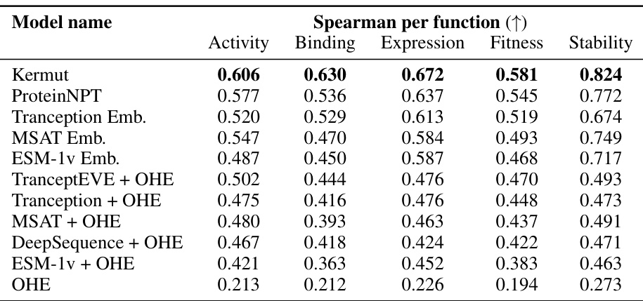
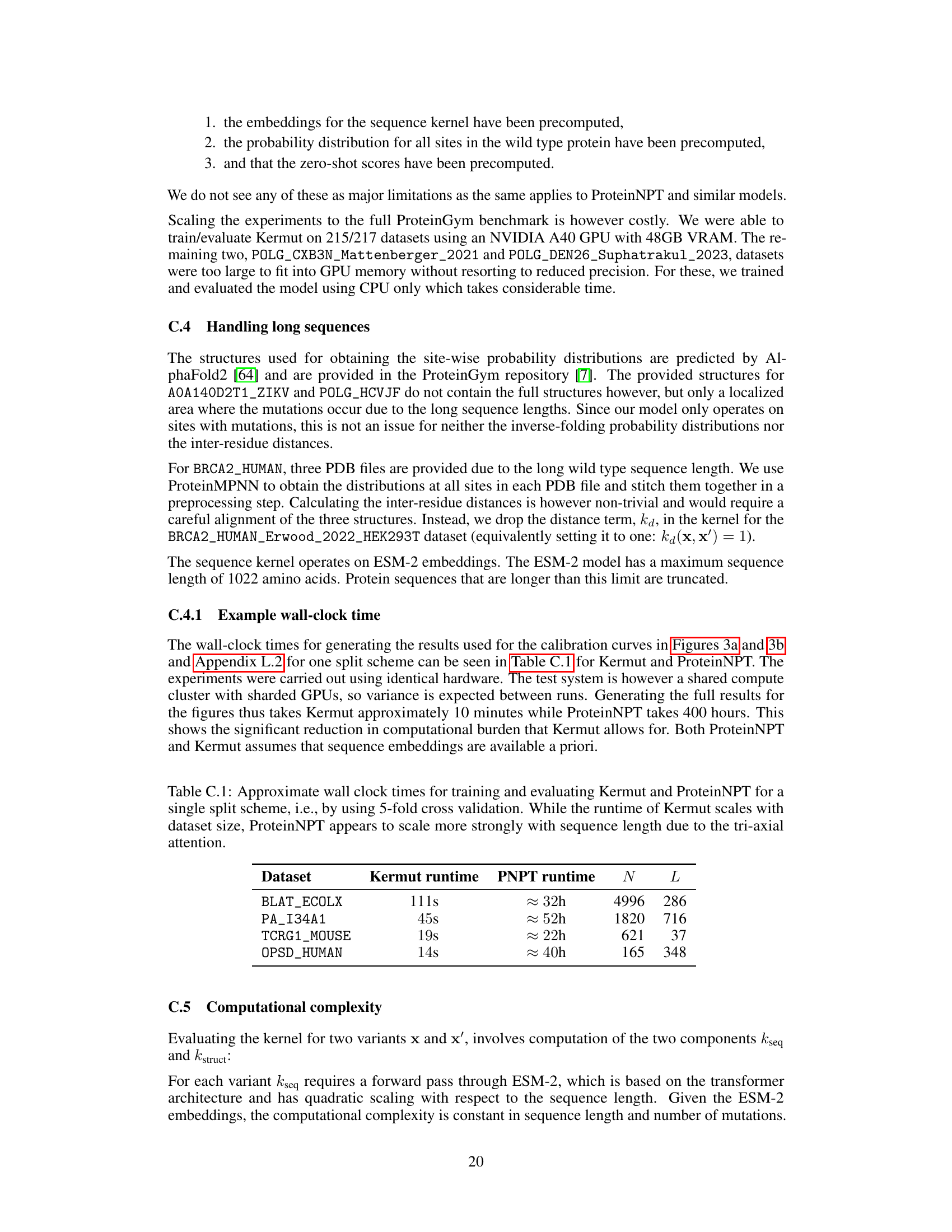
This table presents the results of the Kermut model and other state-of-the-art models on the ProteinGym benchmark. It shows the performance (Spearman correlation and Mean Squared Error) of each model across three different cross-validation schemes (‘Contig’, ‘Mod’, ‘Rand’). The ‘Avg’ column provides the average performance across the three schemes. The table highlights Kermut’s superior performance, particularly in the more challenging ‘Modulo’ and ‘Contiguous’ settings. It also categorizes models by type (one-hot encoding or non-parametric transformer).
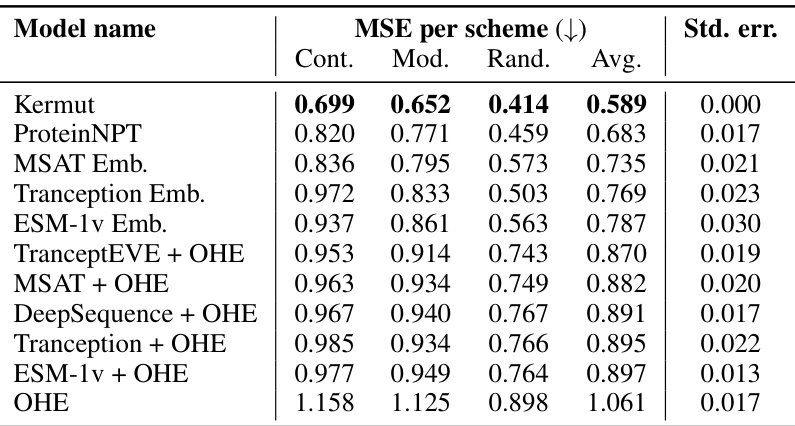
This table presents the performance of Kermut and various other models on the ProteinGym benchmark, which evaluates protein variant effect prediction. It shows the Spearman correlation and Mean Squared Error (MSE) for three different cross-validation schemes: contiguous, modulo, and random. The results are broken down by model type (one-hot encoding or non-parametric transformer) and highlight Kermut’s superior performance, particularly in the more challenging modulo and contiguous settings.
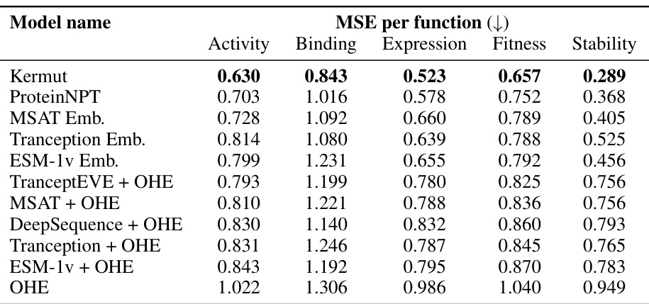
This table presents the performance of Kermut and other state-of-the-art methods on the ProteinGym benchmark. It shows the Spearman correlation and Mean Squared Error (MSE) for three different cross-validation schemes: contiguous, modulo, and random. The results are broken down by model type (one-hot encoding or non-parametric transformer). The best performing model for each metric and scheme is shown in bold, demonstrating Kermut’s superior performance across various settings and its significant improvement in the more challenging contiguous and modulo schemes.

This table presents the performance of the Kermut model and other state-of-the-art models on the ProteinGym benchmark, a comprehensive dataset for evaluating protein variant effect prediction. The results are shown in terms of Spearman correlation and Mean Squared Error (MSE), separately for three different data splits: contiguous, modulo, and random. The table also specifies whether the model uses one-hot encodings (OHE) or non-parametric transformers (NPT) for input representation. Kermut’s superior performance across all splits and the significant improvement for challenging splits (modulo and contiguous) highlight the effectiveness of the proposed approach. The best results for each metric in each split are indicated in bold.
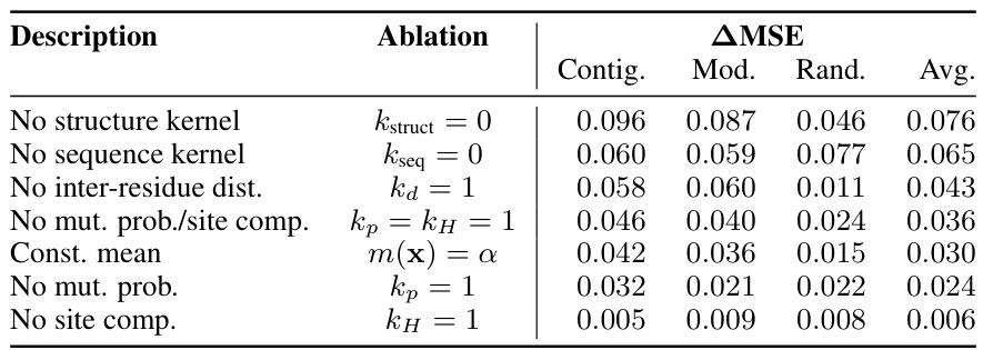
This table presents the results of an ablation study conducted on the Kermut model. Key components of the composite kernel were systematically removed, and the model’s performance was evaluated on a subset of assays from the ProteinGym benchmark. The table shows the changes in Spearman correlation and Mean Squared Error (MSE) resulting from each ablation, compared to the full Kermut model. This allows assessment of the contribution of each kernel component to the model’s overall performance. Negative values indicate a decrease in performance compared to the complete model.
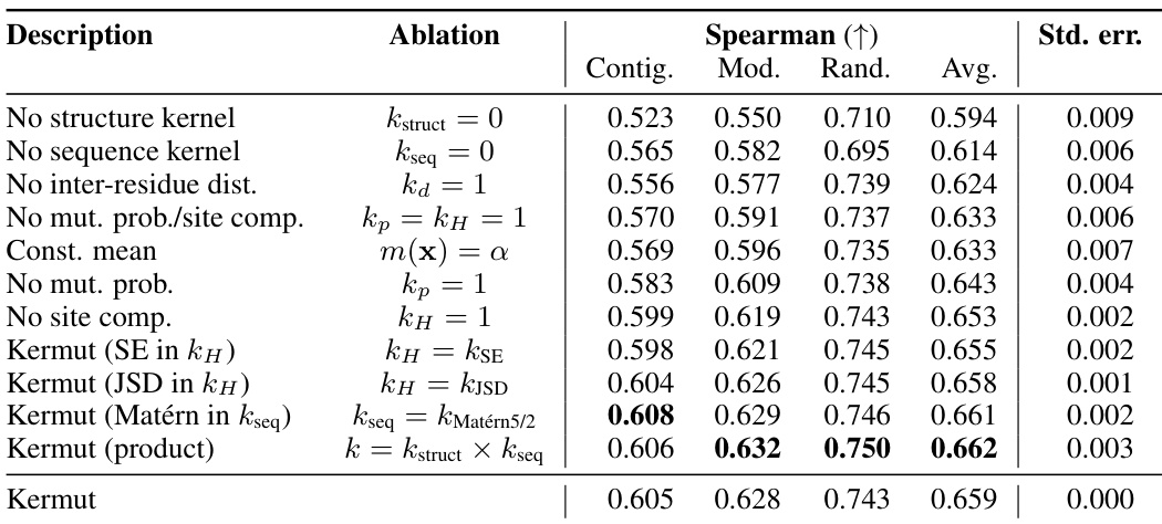
This table presents the performance of the Kermut model and other state-of-the-art models on the ProteinGym benchmark. The benchmark evaluates protein variant effect prediction using three different cross-validation schemes: contiguous, modulo, and random. The table shows the Spearman correlation and Mean Squared Error (MSE) for each model and scheme, indicating Kermut’s superior performance, particularly in the more challenging modulo and contiguous settings. The model types (OHE and NPT) refer to one-hot encoding and non-parametric transformer based models respectively.
This table shows the performance of the Kermut model and other state-of-the-art models on the ProteinGym benchmark, a comprehensive dataset for evaluating protein variant effect prediction. The results are broken down by three different cross-validation schemes (Contig, Mod, Rand), evaluating both Spearman correlation (higher is better) and Mean Squared Error (MSE; lower is better). The table highlights Kermut’s superior performance, particularly in the more challenging ‘modulo’ and ‘contiguous’ settings, and compares its performance to models using one-hot encodings and non-parametric transformers.
This table presents the performance of Kermut and other models on the ProteinGym benchmark for protein variant effect prediction. It shows the Spearman correlation and Mean Squared Error (MSE) across three different cross-validation schemes (contiguous, modulo, random), highlighting Kermut’s superior performance, particularly in the more challenging modulo and contiguous settings. Model types are categorized as one-hot encoding (OHE) or non-parametric transformers (NPT).
This table presents the results of the Kermut model and other state-of-the-art models on the ProteinGym benchmark. It shows the performance (Spearman correlation and Mean Squared Error) broken down by three different cross-validation schemes (contiguous, modulo, random) for evaluating the robustness of the models and comparing them under different conditions. The table also differentiates between model types (One-Hot Encoding and Non-parametric Transformers). Bold values indicate the best-performing model for each metric and scheme.

This table presents the results of the Kermut model and other state-of-the-art models on the ProteinGym benchmark, a comprehensive dataset for evaluating protein variant effect prediction. The table shows the performance of different models across three different cross-validation schemes (Contiguous, Modulo, Random) that test the robustness of the prediction models on different data splits. The metrics reported are Spearman correlation (higher is better) and Mean Squared Error (MSE, lower is better). The table highlights Kermut’s superior performance, particularly in the more challenging Modulo and Contiguous schemes.
This table presents the performance of the Kermut model and other state-of-the-art models on the ProteinGym benchmark. It shows the Spearman correlation and Mean Squared Error (MSE) for three different data split schemes (Contiguous, Modulo, Random) commonly used in protein variant effect prediction tasks. The results are compared for different model types (one-hot encoding and non-parametric transformers). The table highlights Kermut’s superior performance across all split schemes and model types, with particularly large improvements in the more challenging Modulo and Contiguous settings. The best results for each metric are highlighted in bold.

This table presents the results of the Kermut model and several other state-of-the-art models on the ProteinGym benchmark for protein variant effect prediction. The benchmark includes three different cross-validation schemes: contiguous, modulo, and random. The table shows the Spearman correlation and Mean Squared Error (MSE) for each model and scheme. The ‘Contig.’, ‘Mod.’, and ‘Rand.’ columns represent the contiguous, modulo, and random splits, respectively. The ‘Avg.’ column is the average performance across the three splits. The table highlights Kermut’s superior performance across all schemes, particularly in the more challenging modulo and contiguous settings. OHE and NPT refer to one-hot encoding and non-parametric transformer model types, respectively.
Full paper#
