↗ OpenReview ↗ NeurIPS Proc. ↗ Chat
TL;DR#
Deep learning models are vulnerable to adversarial attacks, where small input perturbations drastically change predictions. Existing defenses like Randomized Smoothing (RS) often compromise accuracy or only defend against small attacks. This paper tackles these issues.
The paper proposes Adaptive Randomized Smoothing (ARS), a novel defense that uses a two-step approach. The first step adapts to the input by computing an input-dependent mask, reducing the input dimension and thus noise needed for certification. The second step adds noise and makes a prediction. ARS leverages f-Differential Privacy for rigorous theoretical analysis and adaptive composition of multiple steps. Experiments on CIFAR-10, CelebA, and ImageNet show significant improvements in both standard and certified accuracy compared to existing methods.
Key Takeaways#
Why does it matter?#
This paper is important because it addresses the limitations of existing defenses against adversarial attacks in machine learning. It introduces Adaptive Randomized Smoothing (ARS), a novel method that significantly improves the accuracy and robustness of deep learning models. This work is particularly relevant given the increasing concerns about the vulnerability of AI systems to malicious attacks, opening new avenues for research in certified robustness and adaptive defenses.
Visual Insights#

This figure illustrates the two-step Adaptive Randomized Smoothing (ARS) process for handling L∞-bounded adversarial attacks. The first step (M₁) adds noise to the input (X) and uses a mask model (w) to generate a mask based on the noisy input. This mask focuses on task-relevant information, reducing the input dimension for the next step. The second step (M₂) takes the masked input and adds further noise. Finally, a base classifier (g) processes a weighted average of the outputs from M₁ and M₂ to produce the final prediction. The standard Randomized Smoothing (RS) is a special case of this process where there is no masking step (M₁).
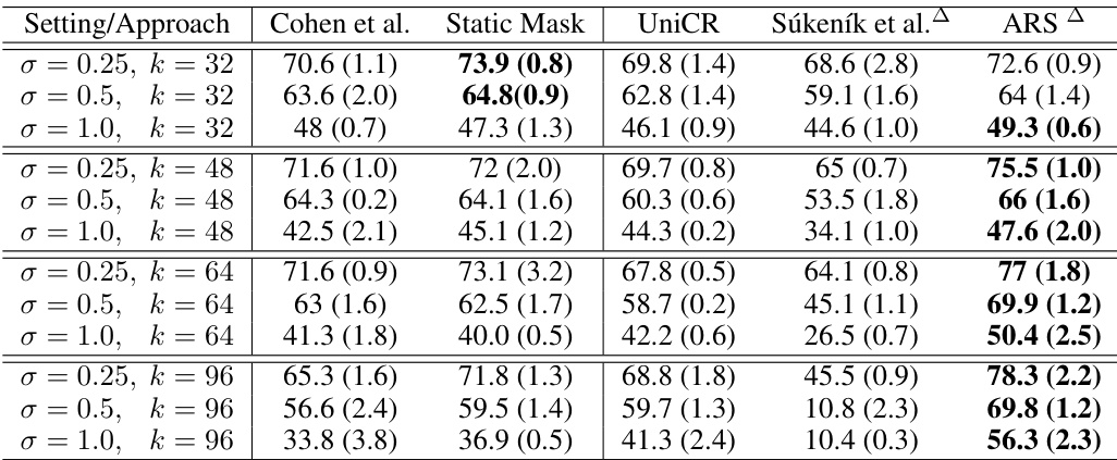
This table presents the standard accuracy (error rate at radius r=0) for different model approaches on the CIFAR-10 dataset with added background images (20kBG benchmark). The table compares several methods: Cohen et al., Static Mask, UniCR, Súkeník et al., and ARS. It shows accuracy results across various noise levels (σ) and input dimensions (k). ARS, an adaptive method, demonstrates higher accuracy in most cases. The full results with more noise levels are in Appendix D.
In-depth insights#
Adaptive RS Theory#
The core idea behind Adaptive Randomized Smoothing (ARS) theory is to rigorously certify the predictions of adaptive test-time models against adversarial attacks. It leverages the connection between randomized smoothing and differential privacy (DP), specifically f-DP, to achieve this. Unlike traditional RS, ARS allows for multi-step, input-dependent adaptations during the test phase. The theory cleverly uses f-DP’s composition theorems to provide end-to-end privacy and robustness guarantees for these adaptive steps. This is a significant advancement because prior adaptive RS methods often lacked rigorous theoretical justification. A key contribution is the demonstration that adaptive composition of Gaussian mechanisms does not increase the required noise level compared to a single step, which directly enables more effective and flexible defenses against L∞ adversaries. The theoretical framework lays the groundwork for creating more robust and accurate multi-step defenses, opening new avenues for improving certified robustness in deep learning models.
f-DP for Robustness#
The concept of f-DP (f-Differential Privacy) for achieving robustness in machine learning models is a significant advancement. It leverages the theoretical framework of DP but enhances it by focusing on the power of hypothesis tests to guarantee privacy. This approach offers a more nuanced understanding of privacy, moving beyond simple epsilon-delta definitions and instead quantifying the level of privacy based on the difficulty of distinguishing between outputs from neighboring inputs. The key advantage is that f-DP can be applied to the analysis of complex multi-step processes. This is important for adaptive defenses, where the defense mechanism changes based on the input. Unlike traditional DP analysis which often struggles with adaptive composition, f-DP’s ability to handle adaptive steps makes it suitable for rigorously certifying the robustness of such systems. By relating adaptive randomized smoothing to f-DP, it becomes possible to offer rigorous certified accuracy bounds, even in scenarios where the defense strategy itself evolves dynamically. This leads to improved accuracy and stronger robustness guarantees, which is a crucial step in deploying more resilient and trustworthy machine learning models in real-world applications.
Multi-step Defense#
The concept of “Multi-step Defense” in adversarial robustness signifies a paradigm shift from single-stage defense mechanisms. Instead of relying on a single defensive layer, multi-step defenses employ a sequence of techniques to iteratively mitigate adversarial attacks. This approach acknowledges the adaptive nature of attacks, where adversaries may strategically modify their approach based on the observed defenses. By cascading multiple defensive steps, the overall robustness and security of the model can be significantly enhanced. Each step aims to reduce the effectiveness of attacks while maintaining satisfactory accuracy. However, the design and analysis of multi-step defenses require careful consideration of the interactions between the individual steps; improper sequencing can even result in decreased resilience. Certified robustness guarantees for multi-step defenses pose a significant theoretical challenge, as the composition of multiple steps needs to be rigorously analyzed. Further research needs to address this theoretical gap and investigate the trade-off between enhanced security and increased computational complexity inherent to these multi-step mechanisms. Adaptive approaches, where the defense adapts to the specific characteristics of the input, offer a promising avenue in multi-step defenses; allowing for more flexible and tailored defense strategies, as seen in techniques like Adaptive Randomized Smoothing (ARS).
L∞-bounded Attacks#
L∞-bounded attacks represent a significant challenge in adversarial machine learning, focusing on small, targeted perturbations to input data. Unlike L2 attacks which consider the magnitude of the overall change, L∞ attacks constrain the maximum change at any single data point. This makes them more difficult to detect as they can easily evade simple defenses relying on magnitude thresholds. The paper’s focus on L∞-bounded attacks is crucial because of their practical relevance. Real-world adversarial examples often have this characteristic due to physical constraints or limitations on how data can be manipulated. The ability to certify robustness against these attacks, as explored in the research, is therefore essential for deploying machine learning models in safety-critical applications. Furthermore, the theoretical framing of adaptive randomized smoothing (ARS) within the context of L∞ attacks provides a rigorous mathematical foundation, improving upon the existing limitations of non-adaptive approaches. This rigorous framework allows for sound composition of multiple defense steps, leading to enhanced robustness without compromising accuracy.
Future of ARS#
The future of Adaptive Randomized Smoothing (ARS) hinges on addressing its current limitations while exploring new avenues for improvement. Computational cost remains a significant hurdle; future research should focus on optimization techniques to make ARS more practical for large-scale deployments. Extending ARS’s applicability beyond the L∞ norm to other threat models, such as L2 or L1, is crucial for broader impact. Furthermore, combining ARS with other defense mechanisms, like adversarial training or data augmentation, could yield even more robust certified accuracy. Investigating the theoretical underpinnings of ARS within the framework of differential privacy promises further insights into composition results and robustness guarantees. Addressing the challenges associated with high-dimensional inputs will also be key, possibly through improved masking techniques or more efficient dimensionality reduction methods. Finally, rigorous empirical evaluations on a wider range of datasets and tasks are essential to establish ARS’s true effectiveness and robustness in real-world scenarios.
More visual insights#
More on figures

This figure illustrates the two-step Adaptive Randomized Smoothing (ARS) process for handling L∞-bounded adversarial attacks. The first step (M1) adds noise to the input (X) and uses a mask model (w) to process the noisy input into a mask (w(m1)). The second step (M2) takes this masked input (w(m1)X) and adds further noise. Finally, a base classifier (g) processes a weighted average of the outputs from steps M1 and M2 to generate the final prediction. The figure also shows how standard Randomized Smoothing (RS) is a simplified version of ARS.

This figure shows the input images to the model and the corresponding masks generated by the mask model (M1) in the two-step ARS. The left side shows original CIFAR-10 images superimposed with larger background images of varying sizes (k x k pixels), where k represents the dimension of the input. The right side shows the grayscale masks predicted by the mask model (M1) which highlight the relevant parts of the image that are important for classification. The masks are learned end-to-end during training. Appendix D.2 provides more detail about other stages of the ARS architecture for each image shown in this figure.

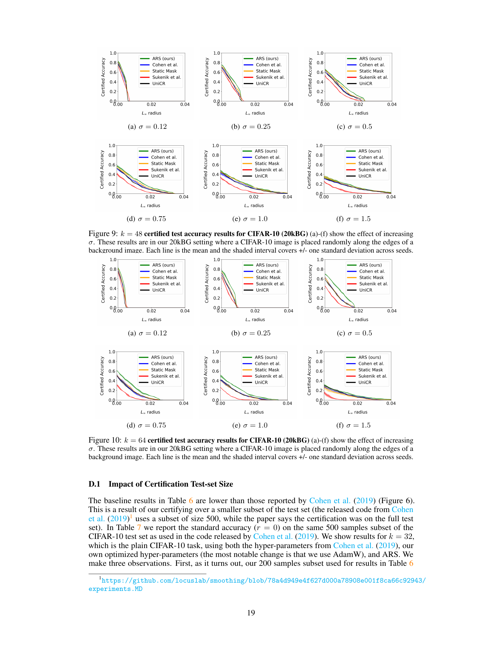
The figure displays the certified test accuracy on CIFAR-10 with distractor backgrounds (20kBG). It shows how certified accuracy changes with different levels of noise (σ) and input dimensionality (k). The plots illustrate the impact of both increased dimensionality and noise on the certified accuracy of different methods, including ARS (Adaptive Randomized Smoothing), Cohen et al. (standard randomized smoothing), static mask, UniCR, and Súkeník et al. ARS shows improved robustness to both higher dimensionality and increased noise levels.
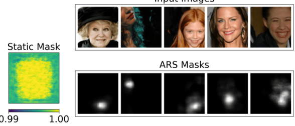
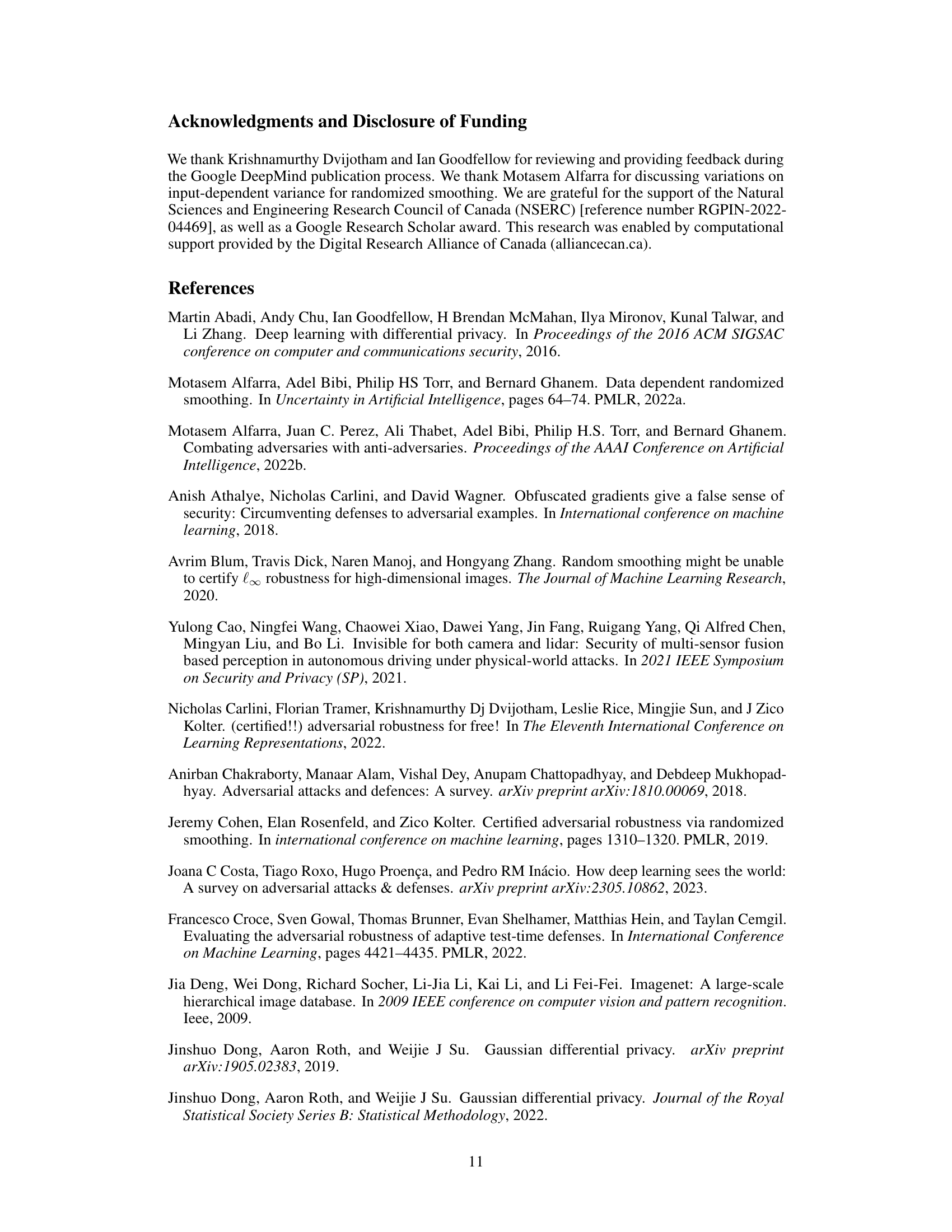
This figure shows the test set images for CelebA benchmark and their corresponding masks generated by ARS and static mask. The static mask is almost uniformly 1 across all pixels, while ARS masks are sparse and localized, focusing on the mouth region in each image.

This figure shows the certified test accuracy of the proposed ARS method on the CIFAR-10 with 20k background dataset. It illustrates how the certified accuracy changes as a function of the L∞ radius of adversarial attacks, for different levels of noise (sigma) and input dimensionality (k). The results demonstrate that ARS outperforms other state-of-the-art methods across a range of settings, highlighting its effectiveness in certifying robustness against adversarial examples.
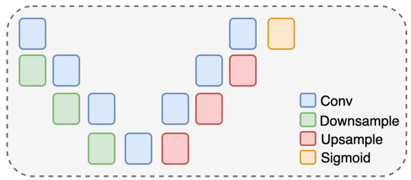
This figure shows the architecture of the Mask model w (M1). It is a UNet architecture which is used to preserve dimensions. It uses a Sigmoid layer at the end of the model to output values between 0 and 1 for mask weights. The hyperparameters of the UNet are: in_channels=3, out_channels=1 (to output a mask), base_channel=32, channel_mult={1,2,4,8}.

This figure displays the certified test accuracy results for the CIFAR-10 dataset with 20k background images (20kBG). It shows how certified accuracy changes with different levels of noise (σ) and input dimensionality (k). The plots illustrate the impact of increasing dimensionality (by adding background noise) and increasing noise levels on the certified accuracy of different defense methods. Each line represents the mean certified accuracy across multiple runs, with shaded areas indicating the standard deviation.
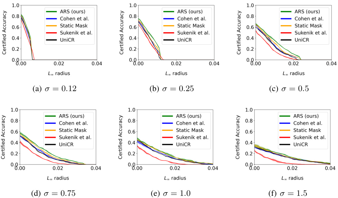
This figure displays the certified test accuracy results on the CIFAR-10 dataset with 20k background images, also known as CIFAR-10 (20kBG), for different dimensionality (k) and noise levels (σ). The graphs illustrate how the certified accuracy changes with different levels of L∞ radius for various methods: ARS, Cohen et al., Static Mask, UniCR, and Súkeník et al. The results show that ARS consistently performs better in most cases.
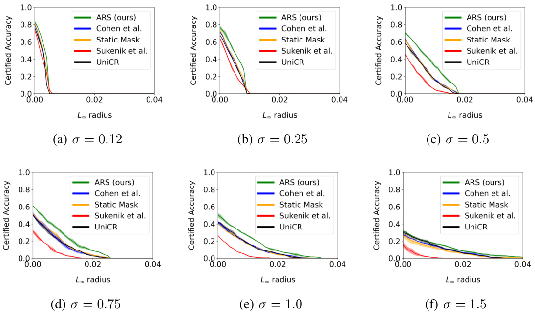
This figure shows the certified test accuracy results on the CIFAR-10 dataset with distractor backgrounds (20kBG). The plots illustrate how certified accuracy changes with different levels of noise (σ) and input dimensionality (k). The experiment evaluates the impact of both higher dimensionality and higher noise levels on the performance of the Adaptive Randomized Smoothing (ARS) method and baseline methods (Cohen et al., Static Mask, UniCR, and Sukenik et al.).

This figure displays the certified test accuracy results for the CIFAR-10 dataset with distractor backgrounds (20kBG). It illustrates how both the dimensionality (k) and noise level (σ) affect the accuracy of different methods: ARS (Adaptive Randomized Smoothing), Cohen et al. (standard Randomized Smoothing), Static Mask (a baseline), Súkeník et al. (a test-time adaptive variance method), and UniCR (a test-time adaptive noise distribution method). The graphs show that ARS consistently outperforms other methods, particularly as dimensionality increases. This demonstrates the effectiveness of ARS in handling high-dimensional inputs and achieving certified robustness.
This figure illustrates the two-step adaptive randomized smoothing (ARS) process for handling L∞-bounded adversarial attacks. The first step (M1) adds noise to the input (X) and uses a mask model (w) to process the noisy input into a mask (w(m1)). The second step (M2) takes the masked input (w(m1)X) and adds more noise to produce m2. Finally, a base classifier (g) processes a weighted average of m1 and m2 to generate the final prediction. The standard randomized smoothing (RS) method is a simplified version where there’s only the second step (M2), without the masking step (M1).

This figure illustrates the two-step Adaptive Randomized Smoothing (ARS) process for handling L∞-bounded adversarial attacks. The first step (M1) adds noise to the input (X) and uses a mask model (w) to process the noisy input into a mask (w(m1)). The second step (M2) takes the masked input (w(m1)X) and adds further noise, resulting in m2. Finally, a base classifier (g) processes a weighted average of m1 and m2 to produce the final prediction. The figure also highlights that standard Randomized Smoothing (RS) is a simplified version of ARS with no M1 step (i.e., w(.) = 1 and only one noise addition).

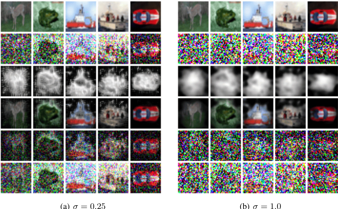
This figure shows example inputs to the model for different values of k (image dimension). The left side shows the original CIFAR-10 image superimposed on a larger background image, making the classification task more challenging. The right side shows the corresponding masks generated by the mask model (M1) in the ARS architecture. These masks highlight the relevant image regions that the model should focus on during classification, effectively reducing the dimensionality of the input to M2 and improving robustness. Appendix D.2 provides more detailed visualization of the different steps in the multi-step ARS architecture.
This figure illustrates the two-step Adaptive Randomized Smoothing (ARS) process for handling L∞-bounded adversarial attacks. The first step (M1) adds noise to the input (X) and uses a mask model to generate a mask (w(m1)) based on the noisy input. This mask focuses the processing on relevant information. The second step (M2) adds noise to the masked input (w(m1)X) and produces m2. Finally, a base classifier (g) combines m1 and m2 to produce the final prediction. The standard Randomized Smoothing (RS) method is a simplified version of ARS, omitting the first masking step.

This figure shows how the adaptive masking in ARS reduces noise in regions relevant to classification. The top row shows example input images. The second row shows the images after the first noise injection step (M1). The third row displays the sparse masks (learned by the mask model) which focus on the mouth region. The bottom row shows the images after the second noise injection and averaging step (M2). The masks effectively reduce noise around the mouth area, improving classification accuracy.
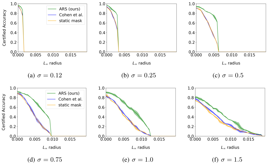
This figure shows the certified test accuracy results for CIFAR-10 with 20k background images dataset. The x-axis represents the L∞ radius, and the y-axis represents the certified accuracy. The figure consists of six subfigures, each showing the results for a different combination of dimensionality (k) and noise level (σ). In each subfigure, different methods are compared: ARS, Cohen et al., static mask, Súkeník et al., and UniCR. The shaded area around each line represents the standard deviation of the results across multiple seeds.

This figure shows how the adaptive masking in ARS reduces noise in areas important for classification. The images follow the architecture in Figure 1. The first query noised images are fed to the mask model, which produces sparse masks concentrated around the object. After the weighted averaging of m1 and m2, the second query noised images show reduced noise around the object.

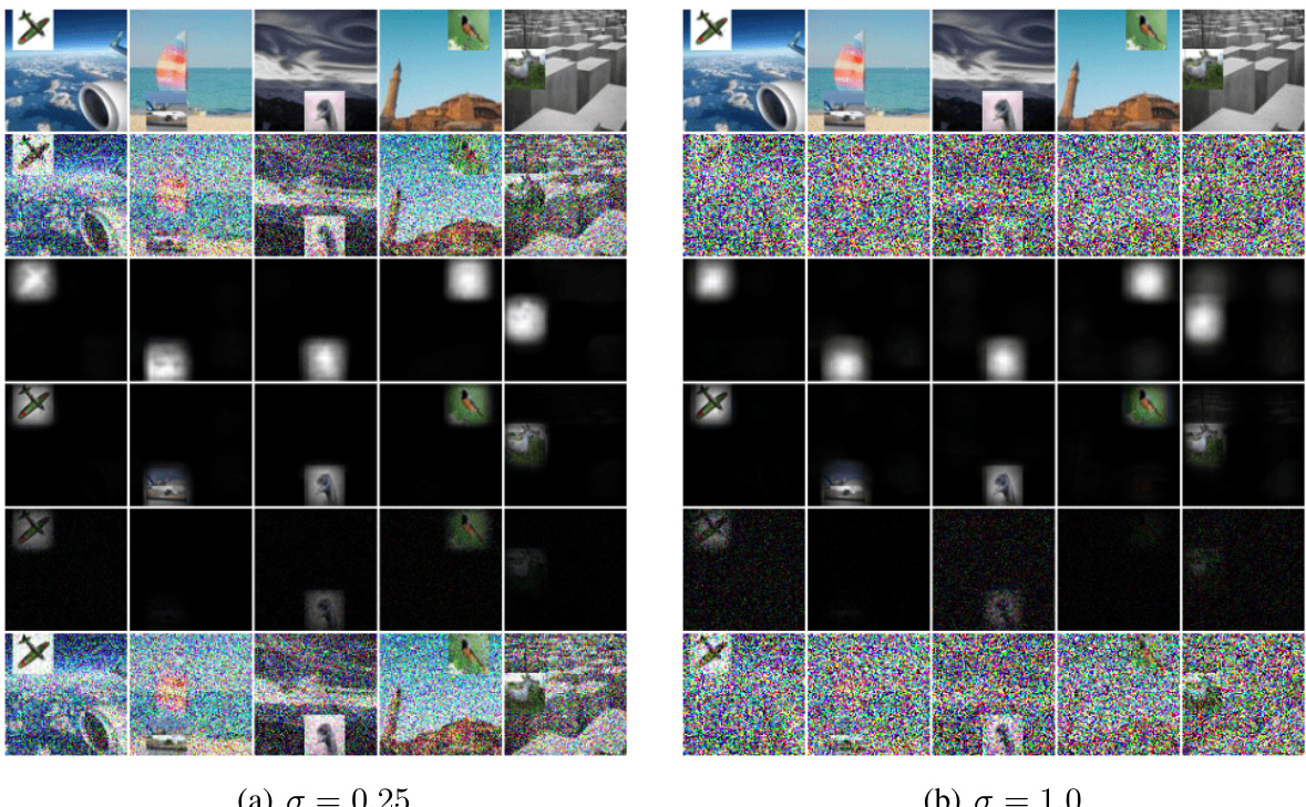
This figure shows the effect of adaptive masking in reducing noise around important areas for classification in ImageNet. The figure presents a sequence of images illustrating different stages in the two-step ARS architecture. The first row shows the original input images. The second row shows the noisy images after the first step (M1) which adds noise. The third row presents the masks generated by the mask model (w), highlighting the important regions. The fourth row displays the noisy images after the second step (M2), where the noise has been reduced in the regions identified by the masks. These images are then combined to obtain the final classification result, showcasing the effectiveness of adaptive masking in improving robustness to adversarial attacks.

This figure illustrates the two-step Adaptive Randomized Smoothing (ARS) process for handling L∞-bounded adversarial attacks. The first step (M1) adds noise to the input (X) and uses a mask model (w) to process the noisy input to generate a mask (w(m1)). The second step (M2) uses the mask from step 1 to process the input again by applying a weighted average of the noisy input from M1 and M2 before generating the output label using the base classifier (g). The standard randomized smoothing (RS) is a simplified version of ARS with no M1 step (i.e., the mask is always 1 and there is only one noise addition).
More on tables

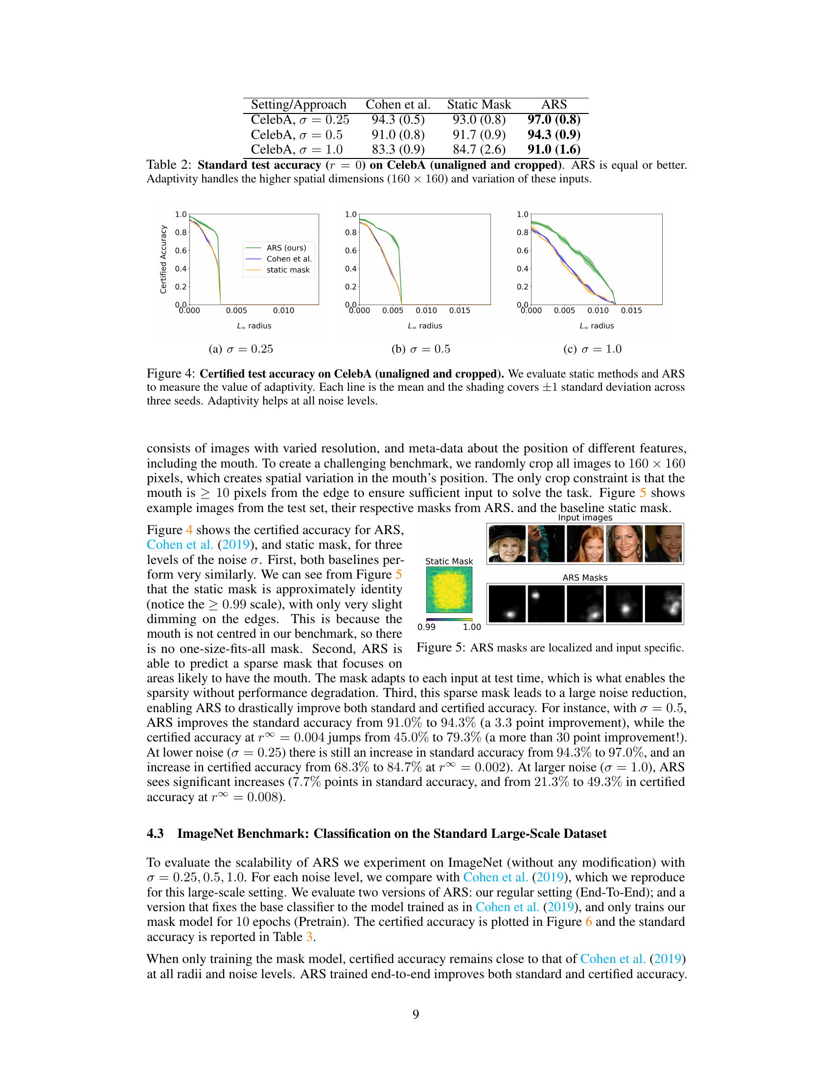
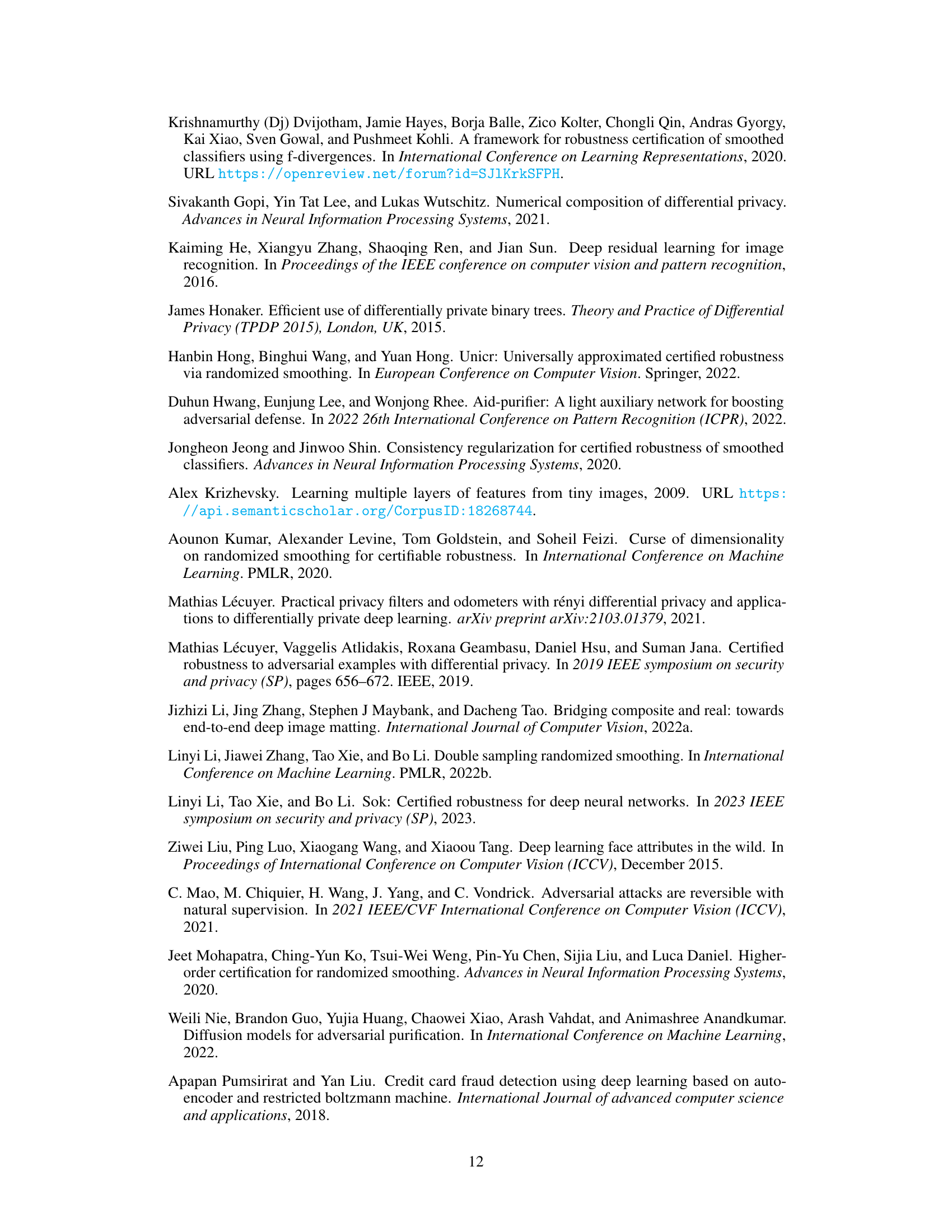
This table presents the standard test accuracy (when the radius r is 0) for three different approaches on the CelebA dataset. The three methods compared are Cohen et al., Static Mask, and ARS (the proposed method). The results are shown for three different noise levels (σ = 0.25, 0.5, and 1.0). The table demonstrates that ARS consistently achieves equal or better accuracy compared to the other two methods, highlighting its ability to handle high spatial dimensions and input variations.

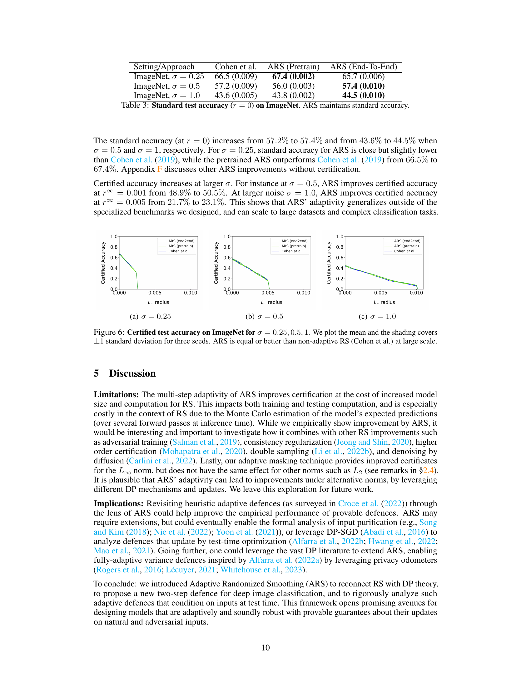
This table presents the standard test accuracy (at radius r=0) on the ImageNet dataset for three different noise levels (σ = 0.25, 0.5, 1.0). It compares the performance of the proposed Adaptive Randomized Smoothing (ARS) method with the standard Randomized Smoothing (RS) method by Cohen et al. Two versions of ARS are shown: one where only the mask model is trained (‘Pretrain’), and another where the entire model is trained end-to-end (‘End-To-End’). The results indicate that ARS maintains a similar standard accuracy to the Cohen et al. method, showcasing its scalability to large datasets.
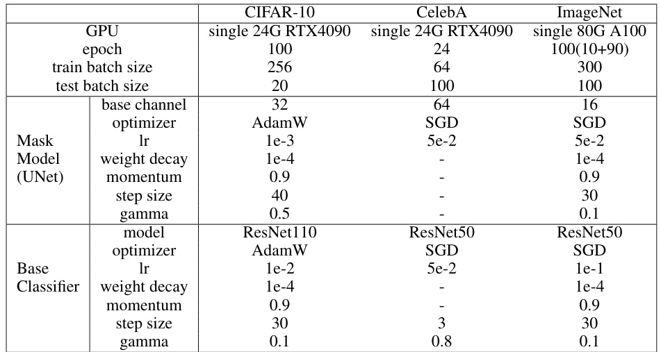
This table lists the hyperparameters used for training the Adaptive Randomized Smoothing (ARS) model. It breaks down the settings for different aspects of the model training process, including for the Mask Model (UNet) and the Base Classifier. Different hyperparameters were used for different datasets (CIFAR-10, CelebA, and ImageNet). The table includes the GPU used, the number of epochs, batch sizes, base channel numbers, optimizers (AdamW and SGD), learning rates, weight decay, momentum, step sizes, and gamma values. Appendix C.3 offers additional details on hyperparameter tuning for CIFAR-10.

This table presents the values of β used for the UniCR method in the experiments. β is a parameter of the generalized normal distribution used for noise in the randomized smoothing technique. The table shows that β was tuned for different values of k (input dimension) and σ (noise level) in the CIFAR-10 BG20k experiment, resulting in slightly different optimal β values for various combinations of k and σ.

This table presents the standard accuracy (with no adversarial attack, r=0) on a modified CIFAR-10 dataset (20kBG) where images are superimposed on larger backgrounds, varying the input dimension (k). The results are shown for different noise levels (σ) and for several methods: Cohen et al. (standard randomized smoothing), Static Mask (a baseline using a fixed mask), UniCR (a test-time adaptive method), Súkeník et al. (another test-time adaptive method), and ARS (the proposed method). The table highlights the improved accuracy of ARS, especially as the input dimension increases. Standard deviations are also included.
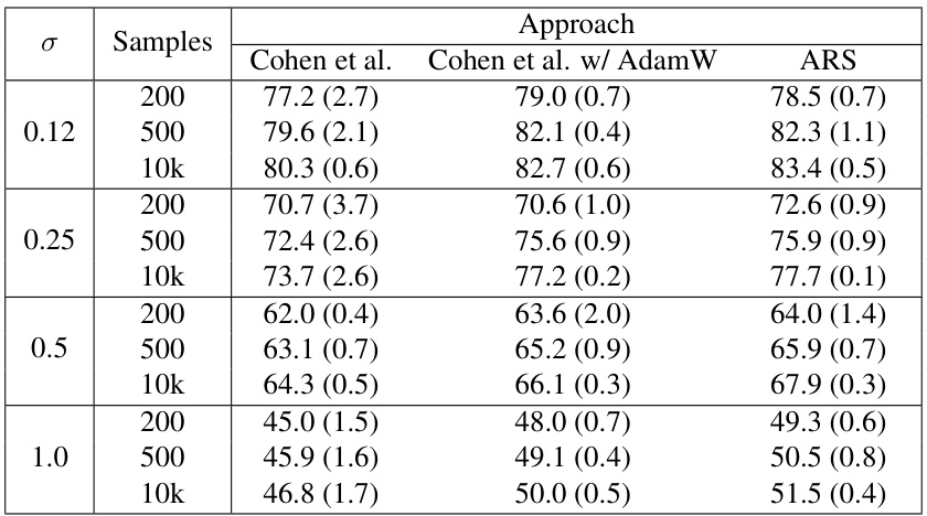
This table presents the standard accuracy (when there is no adversarial attack, r=0) for different model approaches on the CIFAR-10 dataset with 20k background images. It compares the performance of Cohen et al., Static Mask, UniCR, Súkeník et al., and ARS across varying noise levels (σ) and input dimensions (k). The 20kBG benchmark makes the task more challenging by adding distractor background images, highlighting the impact of adaptivity in handling higher dimensional inputs and noise. ARS consistently achieves higher accuracy than other methods.

This table presents the standard test accuracy results for different methods on the CelebA dataset. The accuracy is measured at radius r = 0, meaning no certification is applied. Three methods are compared: Cohen et al., Static Mask, and ARS. The results show that ARS achieves equal or higher accuracy than the other methods. The experiment uses unaligned and cropped CelebA images, which are 160x160 pixels in size, highlighting the impact of adaptivity in handling high spatial dimensions and variations in input images.

This table presents the standard test accuracy (with no certification, r=0) on the ImageNet dataset for three different noise levels (σ = 0.25, 0.5, 1.0). It compares the results of the standard Randomized Smoothing (Cohen et al.) method with two variations of Adaptive Randomized Smoothing (ARS): one where the mask model is pre-trained (ARS (Pretrain)) and one where the entire model is trained end-to-end (ARS (End-To-End)). The table shows that ARS maintains, or slightly improves, the standard accuracy compared to the baseline RS method.
Full paper#


