↗ OpenReview ↗ NeurIPS Proc. ↗ Chat
TL;DR#
Supervised graph prediction (SGP) is challenging due to the complex output space, the absence of suitable loss functions, and the arbitrary size and node ordering of graphs. Existing methods often involve expensive decoding steps or specific assumptions about the input or output data. Many approaches are not fully end-to-end, employing multiple steps or heuristic solutions. These limitations hinder the efficiency and generalizability of SGP models.
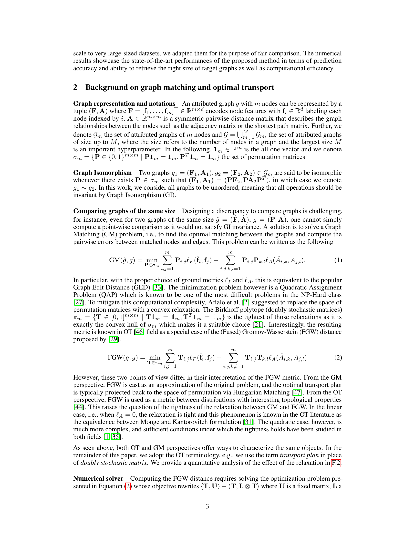
This paper introduces Any2Graph, a novel framework addressing these challenges. It employs a novel Optimal Transport loss, the Partially Masked Fused Gromov-Wasserstein (PMFGW), which is permutation-invariant and fully differentiable. Any2Graph also demonstrates versatility by handling diverse input modalities and outperforming competitors on various datasets, including a novel synthetic dataset (Coloring). The size-agnostic nature of PMFGW further enhances the framework’s flexibility and efficiency.
Key Takeaways#
Why does it matter?#
This paper is important because it introduces Any2Graph, a novel framework for end-to-end supervised graph prediction, addressing the challenges of handling graphs of arbitrary size and node ordering. It presents a new Optimal Transport-based loss function that is both permutation-invariant and differentiable. This advances the field by offering a more versatile and efficient approach to graph prediction tasks across various domains. This work opens avenues for future research in developing more efficient and accurate graph prediction models, particularly in areas like drug discovery and computer vision. The synthetic dataset created also offers a valuable benchmark for comparing SGP methods.
Visual Insights#

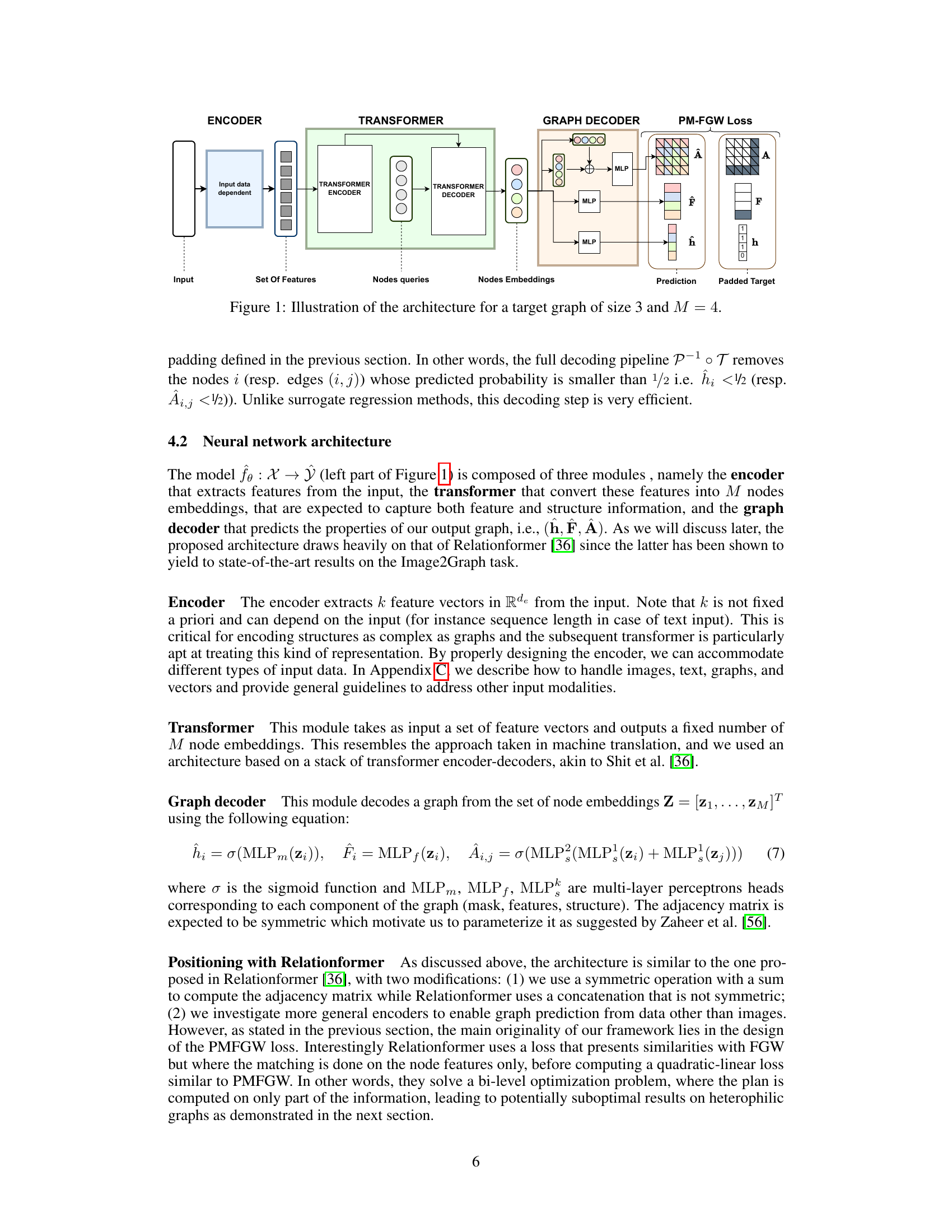
This figure illustrates the Any2Graph architecture, which consists of three main modules: an encoder (input-data-dependent), a transformer (with encoder and decoder), and a graph decoder. The encoder processes the input data and generates a set of features. These features are passed to the transformer, which converts them into node embeddings. The graph decoder then uses these embeddings to predict the properties of the output graph, including the node mask (ĥ), node features (Ê), and adjacency matrix (Â). The PM-FGW loss function compares this prediction to the padded target graph (h, F, A), where ‘h’ represents the node mask, ‘F’ represents the node features, and ‘A’ represents the adjacency matrix of the target graph.
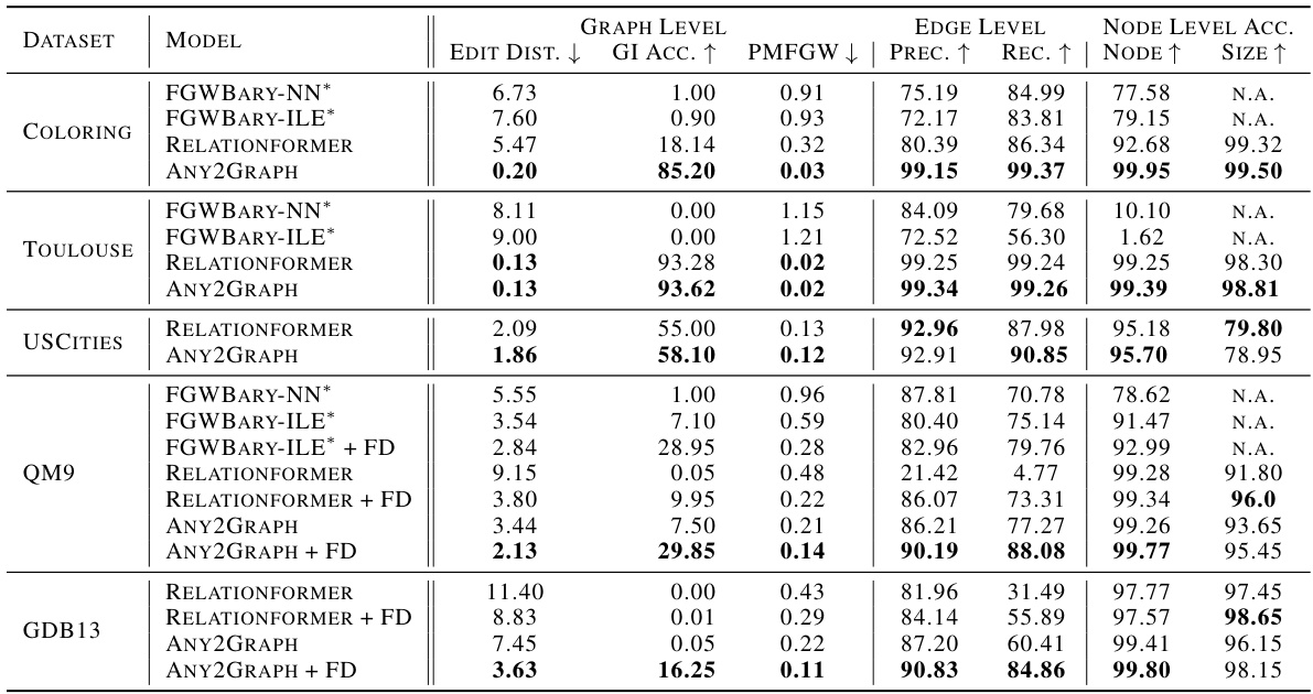
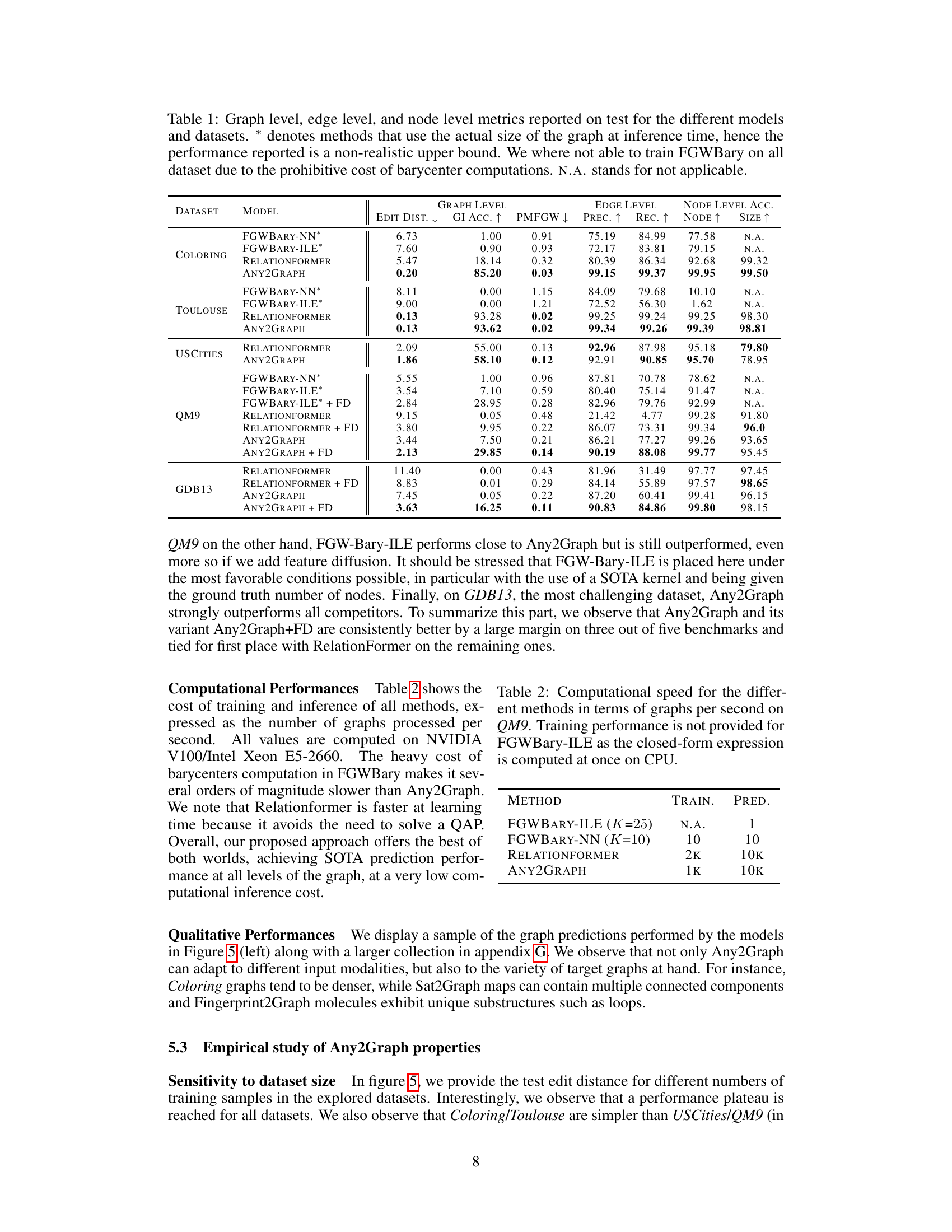
This table presents a comparison of different graph prediction models (FGWBary-NN*, FGWBary-ILE*, Relationformer, Any2Graph) across five datasets (Coloring, Toulouse, USCities, QM9, GDB13). It evaluates model performance using graph-level metrics (Edit Distance, GI Accuracy, PMFGW), edge-level metrics (Precision, Recall), and node-level metrics (Node Accuracy, Size Accuracy). The asterisk (*) indicates that some methods used the true graph size during inference, providing an unrealistic upper bound on performance. Note that FGWBary was not always able to be trained due to computational cost.
In-depth insights#
Optimal Transport Loss#
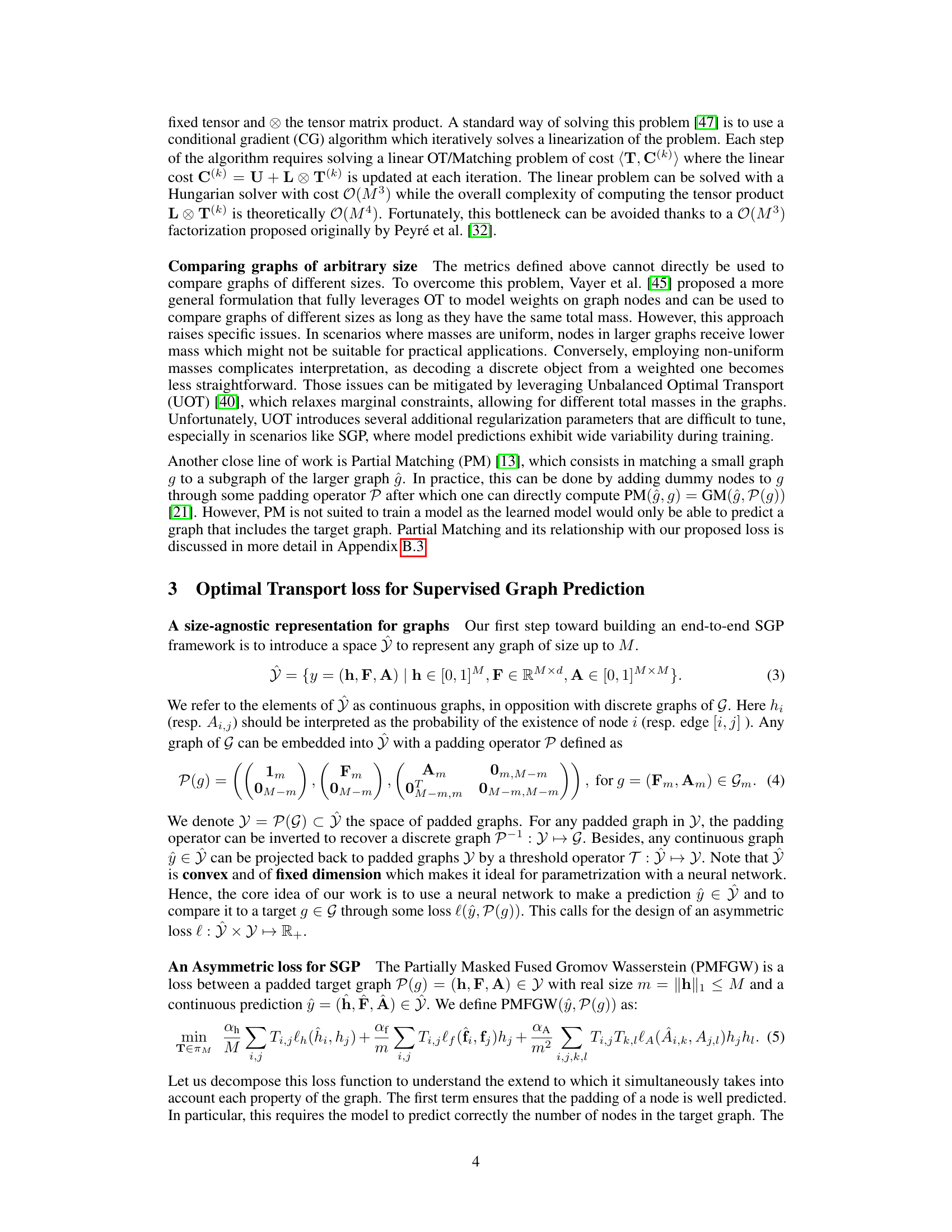
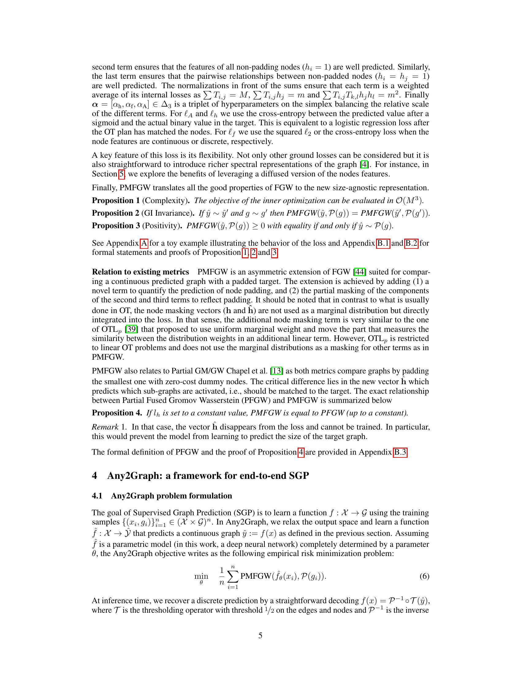
The paper introduces a novel optimal transport loss function, Partially Masked Fused Gromov-Wasserstein (PMFGW), designed for supervised graph prediction. Unlike previous methods, PMFGW addresses the challenges of varying graph sizes and node orderings by incorporating a masking mechanism and handling continuous graph representations. This approach ensures permutation invariance and differentiability, crucial properties for effective training in deep learning settings. PMFGW’s flexibility allows it to adapt to various input modalities and graph structures. The experimental results demonstrate PMFGW’s superiority over existing methods, highlighting its effectiveness in handling diverse graph prediction tasks. The authors also discuss the computational complexity and propose future improvements for larger graphs.
Any2Graph Framework#
The Any2Graph framework presents a novel approach to supervised graph prediction (SGP), addressing the limitations of existing methods. It leverages a size-agnostic graph representation, allowing it to handle graphs of varying sizes without explicit size constraints. The core innovation lies in its use of a novel loss function, Partially Masked Fused Gromov-Wasserstein (PMFGW), which is fully differentiable and permutation invariant. This enables end-to-end training of the model, avoiding the expensive decoding steps found in many traditional approaches. Any2Graph’s modular design incorporates various encoders adaptable to different input modalities (images, text, etc.), making it highly versatile. The framework’s ability to predict both the structure and attributes of graphs makes it suitable for diverse real-world applications. However, the cubic computational complexity of the PMFGW calculation is a major limitation, hindering its scalability to very large graphs. Future improvements could focus on more efficient OT solvers to overcome this limitation and further enhance Any2Graph’s capabilities.
Synthetic Dataset#
The utilization of synthetic datasets in research offers several key advantages. Firstly, they enable researchers to control the complexity and characteristics of the data, ensuring that experiments are conducted under well-defined conditions and allowing for a more targeted evaluation of the proposed methods. Secondly, synthetic datasets can be generated in large quantities, providing a massive amount of data for training and testing deep learning models, which often require huge amounts of data to achieve optimal performance. Thirdly, synthetic data is readily available and avoids privacy concerns, eliminating the complexities and ethical considerations associated with obtaining and utilizing real-world data that might contain sensitive or protected information. Fourthly, they provide flexibility and adaptability, allowing researchers to easily modify and customize their datasets to accommodate specific research needs or test different scenarios. However, a key limitation is that synthetic data might not fully capture the intricate complexities and nuanced patterns of real-world data, potentially leading to overfitting or inaccurate results when applied to real-world problems. Therefore, it is crucial to use synthetic datasets judiciously and in conjunction with real-world data whenever possible, to ensure the robustness and generalizability of research findings.
Scalability Limits#
The scalability of the proposed Any2Graph model is limited by the cubic computational complexity of the optimal transport solver, specifically the Partially Masked Fused Gromov-Wasserstein (PMFGW) loss calculation. This scaling, O(k(M)M³), where M is the maximum graph size and k(M) the number of iterations needed for convergence, prevents efficient handling of large graphs. Feature diffusion is shown to mitigate the cubic complexity somewhat by reducing k(M), but the fundamental limitation persists. While promising strategies like entropic regularization or low-rank OT solvers are suggested for future work to improve scalability, they are not implemented in the current version of Any2Graph. This limitation is a crucial consideration because it restricts the applicability of the method to graphs with relatively few nodes, impacting its real-world usage where larger graphs are common. Therefore, while achieving state-of-the-art performance on the tested datasets, further research is essential to overcome this scalability bottleneck and broaden Any2Graph’s applicability.
Future Directions#
The paper’s core contribution is Any2Graph, a novel framework for end-to-end supervised graph prediction (SGP). A key limitation, however, is scalability to larger graphs. Future work could focus on leveraging spectral graph theory techniques to capture higher-order interactions and improve scalability. This might involve incorporating diffusion on the adjacency matrix or exploring low-rank optimal transport (OT) solvers. Another promising avenue is accelerating the OT solver itself, perhaps through parallelization on GPUs or via approximations. Beyond scalability, investigating the model’s robustness to noisy or incomplete input data and extending it to handle dynamic graph evolution would be valuable. Furthermore, exploring different architectures for the encoder module could enhance its versatility and allow it to effectively process a wider variety of input modalities. Finally, a thorough comparative analysis against a broader range of existing SGP methods on a larger, more diverse set of benchmark datasets would strengthen the validation of Any2Graph’s capabilities and address the limitations of the current empirical study.
More visual insights#
More on figures
The figure illustrates the Any2Graph architecture. It consists of three main modules: an encoder that extracts features from the input data, a transformer that converts these features into node embeddings, and a graph decoder that predicts the properties of the output graph. The output graph’s properties, including node features, adjacency matrix, and node masks, are predicted using multi-layer perceptrons (MLPs). The Partially Masked Fused Gromov-Wasserstein (PMFGW) loss is used to compare the predicted graph with the target graph, considering node permutation invariance and handling graphs of varying sizes. The encoder is designed to be adaptable to different input modalities, making Any2Graph a versatile framework for end-to-end supervised graph prediction.
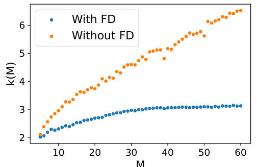
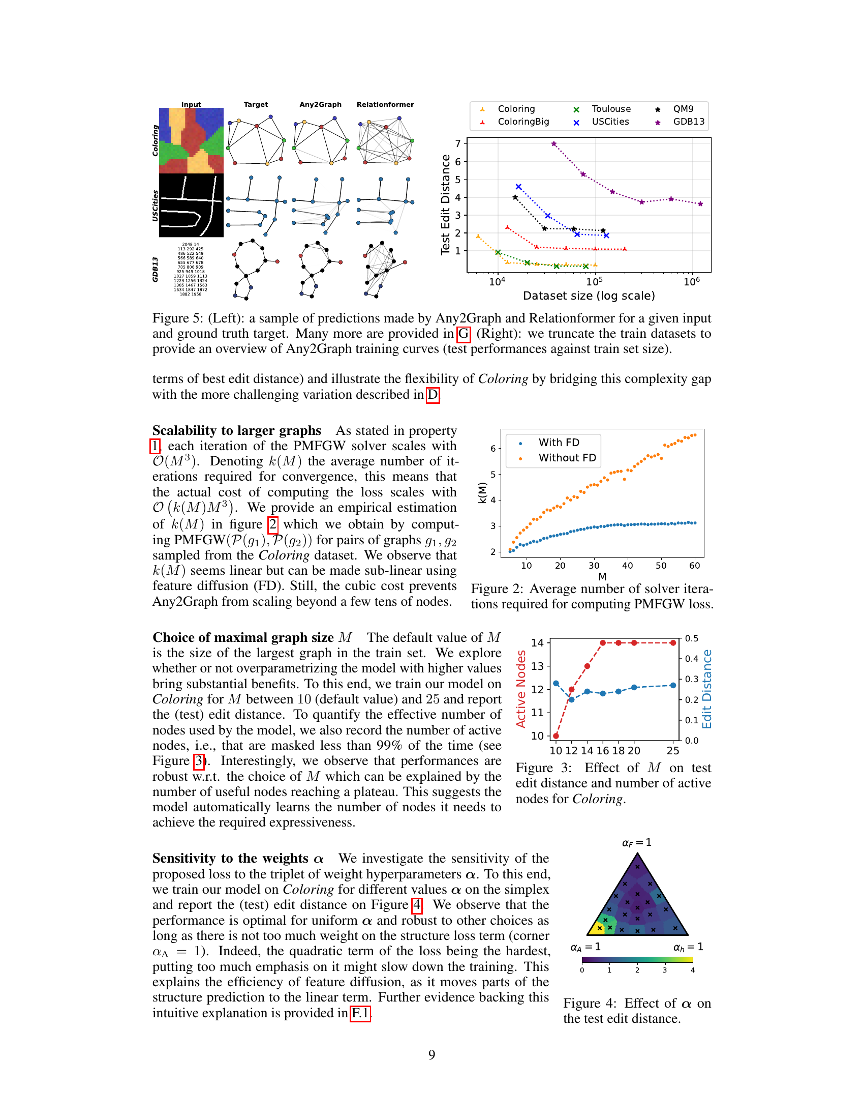
This figure shows the average number of iterations required for the PMFGW solver to converge as a function of the maximum graph size (M). It demonstrates that while the number of iterations increases with M, the increase is slower when feature diffusion (FD) is applied, suggesting a sub-linear relationship between iterations and M in that case.
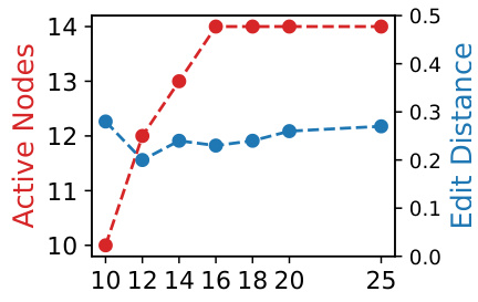
This figure shows the impact of the maximal graph size parameter M on the Any2Graph model’s performance and efficiency for the Coloring dataset. The x-axis represents different values of M, while the left y-axis shows the number of active nodes (nodes with a predicted probability above 0.99), and the right y-axis displays the test edit distance. As M increases, the number of active nodes initially rises sharply before plateauing; suggesting that Any2Graph efficiently utilizes more node embeddings when available. Notably, performance remains robust despite overparameterization, indicating that the model does not overfit.

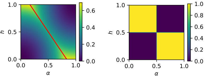
The figure shows the sensitivity analysis of the PMFGW loss to the triplet of weight hyperparameters α = [αh, αf, αA]. The heatmap visualizes the test edit distance obtained for various combinations of αh, αf, and αA on the Coloring dataset. It shows that performance is optimal when αh = αf = αA = 1/3, showing relative robustness to the choice of α.
This figure illustrates the Any2Graph architecture. The architecture consists of three main modules: an encoder, a transformer, and a graph decoder. The encoder takes input data (which can vary depending on the task, such as images, text, or other features) and converts it into a set of features. This feature set is then passed to a transformer module. The transformer processes these features, creating node embeddings which capture both feature and structural information. Finally, the graph decoder module uses these node embeddings to predict the properties of the output graph, including the node features, adjacency matrix, and node masking. The predicted graph and a padded version of the target graph are then fed into the PM-FGW loss function, which measures the difference between them.

This figure illustrates the Any2Graph architecture. It shows the flow of data from the input through three main modules: the encoder, the transformer, and the graph decoder. The encoder processes various input types (images, text, graphs, vectors) to extract features. These features are fed into the transformer which converts them into a fixed number (M) of node embeddings, representing features and structure. The graph decoder uses the node embeddings to generate the predicted graph, including node features, edge weights (adjacency matrix), and the number of nodes (mask). Finally, the Partially-Masked Fused Gromov-Wasserstein (PMFGW) loss compares the predicted continuous graph to the padded target graph.

This figure illustrates the Any2Graph architecture. The input data is first processed by an encoder, specific to the input modality (images, text, etc.). This encoder output is fed into a transformer module which generates node embeddings. These embeddings are then input to a graph decoder, which predicts the structure and features of the output graph. The final output is then compared to the padded target graph using the PMFGW loss. The figure highlights the key components of the model, showing the flow of information from the input to the final output and the role of the PMFGW loss function in guiding the learning process.

This figure shows the architecture of Any2Graph. The input data is processed by an encoder that produces a set of features. Then, a transformer converts these features into M node embeddings. Finally, a graph decoder predicts the properties of the output graph, i.e., (ĥ, F, Â). The whole framework is optimized using the PMFGW loss.

This figure illustrates the Any2Graph architecture. It shows the three main modules: an encoder (input-dependent), a transformer, and a graph decoder. The encoder processes the input data (which can vary depending on the task, such as images or text), and produces a set of features. These features are then processed by a transformer to generate node embeddings. Finally, the graph decoder uses these embeddings to predict the properties of the output graph, including the node features, adjacency matrix, and node mask (which indicates whether a node is present in the graph). The Partially Masked Fused Gromov-Wasserstein (PMFGW) loss function compares the prediction to the padded target graph. The architecture’s flexibility is highlighted by its capacity to handle various input data types.

The figure shows the training curves (test loss vs epochs) for the GDB13 dataset with and without using Hungarian matching during the training process. It demonstrates that using Hungarian matching (projecting the optimal transport plan to the set of permutations) leads to slightly worse performance (higher loss) and more unstable training dynamics (more oscillations). The authors suggest that this is because a continuous transport plan offers a more stable gradient than a discrete permutation.

This figure illustrates the Any2Graph architecture. It consists of three main modules: an encoder that processes the input data (which can vary in type), a transformer that generates node embeddings, and a graph decoder that predicts the output graph structure and features using the PMFGW loss function. The encoder’s design is adaptable based on the input modality. The transformer module processes the node embeddings to consider relationships between nodes. The graph decoder then takes these embeddings to predict the graph’s structure (adjacency matrix) and node features. The overall output is compared to the ground truth using the Partially Masked Fused Gromov-Wasserstein (PMFGW) loss, which is designed to handle variable-sized graphs and is invariant to node permutations.

This figure illustrates the Any2Graph architecture, showing the flow of information from input data through the encoder, transformer, and graph decoder to generate a predicted graph. The input is processed by an input-dependent encoder, followed by a transformer to process the feature vectors. The output of the transformer is then fed into a graph decoder to predict the node features (F), node existence (h), and adjacency matrix (A). The PM-FGW loss function compares the predicted graph with a padded target graph to train the model. The architecture is designed to be adaptable to various input modalities by changing the encoder.
This figure illustrates the Any2Graph architecture, which consists of three main modules: an encoder, a transformer, and a graph decoder. The encoder processes the input data (which can vary depending on the task, such as images or text), and outputs a set of features. These features are then processed by the transformer, which produces a fixed number (M) of node embeddings. Finally, these embeddings are fed to the graph decoder, which predicts the properties of the output graph, such as the node features, the adjacency matrix, and the node mask (indicating whether a node exists in the target graph). The output is then compared against the target graph using the PMFGW loss function.

This figure shows the architecture of Any2Graph, which consists of three main modules: an encoder, a transformer, and a graph decoder. The encoder takes as input different types of data and extracts features. The transformer then converts these features into node embeddings. Finally, the graph decoder predicts the properties of the output graph, including node features and the adjacency matrix. The PM-FGW loss function is used to compare the predicted graph with the target graph. The figure highlights the flow of information through the model, from input data to the final prediction, emphasizing the use of transformers and a novel loss function designed for end-to-end supervised graph prediction.
More on tables
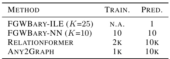
This table presents a comparison of different graph prediction methods across five datasets, evaluating performance using various graph-level, edge-level, and node-level metrics. It highlights the trade-off between performance and the computational cost of methods that require knowledge of the graph size a priori.

This table presents a comparison of different graph prediction models (Any2Graph, Relationformer, FGWBary-NN*, FGWBary-ILE*) on five datasets (Coloring, Toulouse, USCities, QM9, GDB13). It shows the performance of each model using several metrics at different granularities: graph level (edit distance, GI accuracy, PMFGW loss), edge level (precision, recall), and node level (node accuracy, size accuracy). The * indicates methods that unrealistically use the true graph size during inference. Some methods are marked N.A. (not applicable) because they could not be trained on all datasets due to computational cost.

This table presents a comparison of different graph prediction methods (Any2Graph, Relationformer, FGW-Bary-NN, FGW-Bary-ILE) across five datasets (Coloring, Toulouse, USCities, QM9, GDB13). The comparison uses multiple metrics evaluating performance at the graph, edge, and node levels. The asterisk (*) indicates that some methods use the actual graph size at inference time, which is unrealistic. Note that FGW-Bary could not be trained on all datasets due to computational cost.

This table presents a comparison of different graph prediction methods on five datasets. For each dataset and method, it reports graph-level metrics (edit distance, GI accuracy, PMFGW loss), edge-level metrics (precision, recall), and node-level metrics (node accuracy, size accuracy). The table highlights the superior performance of Any2Graph, especially considering its efficiency and ability to handle graphs of arbitrary size.

This table presents a comparison of different graph prediction methods across five datasets. For each dataset and method, it reports graph-level metrics (edit distance, graph isomorphism accuracy, and PMFGW loss), edge-level metrics (precision and recall), and node-level metrics (node accuracy and size accuracy). The table highlights the superior performance of Any2Graph and indicates computational limitations of other methods.

This table compares the performance of different graph prediction models (Any2Graph, Relationformer, FGW-Bary-NN, FGW-Bary-ILE) on five different datasets (Coloring, Toulouse, USCities, QM9, GDB13) using various metrics. The metrics assess performance at the graph, edge, and node levels, offering a comprehensive evaluation of model accuracy. Note that some methods use the graph’s true size during inference, leading to potentially inflated results, while others couldn’t be trained on all datasets due to high computational demands.
This table presents a comparison of different graph prediction models across five datasets, evaluating performance at the graph, edge, and node levels. Metrics include edit distance, graph isomorphism accuracy, PMFGW loss, precision, recall, node accuracy, and size accuracy. The table highlights the superior performance of Any2Graph compared to other methods, while also noting limitations in training certain methods on all datasets due to computational costs.
This table presents a comparison of different graph prediction models on five datasets. It evaluates performance using various graph-level, edge-level, and node-level metrics. The asterisk (*) indicates methods that require knowing the graph’s size beforehand, which is unrealistic in real-world scenarios. The ‘N.A.’ entries signify that results could not be obtained due to computational limitations.
Full paper#


