Parsimony or Capability? Decomposition Delivers Both in Long-term Time Series Forecasting

↗ OpenReview ↗ NeurIPS Proc. ↗ Chat

TL;DR

#

Key Takeaways

#

Why does it matter?

#

This paper is crucial because it challenges the prevailing trend in long-term time series forecasting (LTSF) of increasing model complexity and demonstrates that decomposition methods, particularly the proposed SSCNN model, can achieve superior performance with significantly fewer parameters. This addresses the critical issue of model scalability and computational cost, a major obstacle in applying advanced LTSF models to real-world applications. Furthermore, the paper provides a rigorous analysis comparing decomposition and patching techniques, offering valuable insights for future research in LTSF model design.

Visual Insights

#

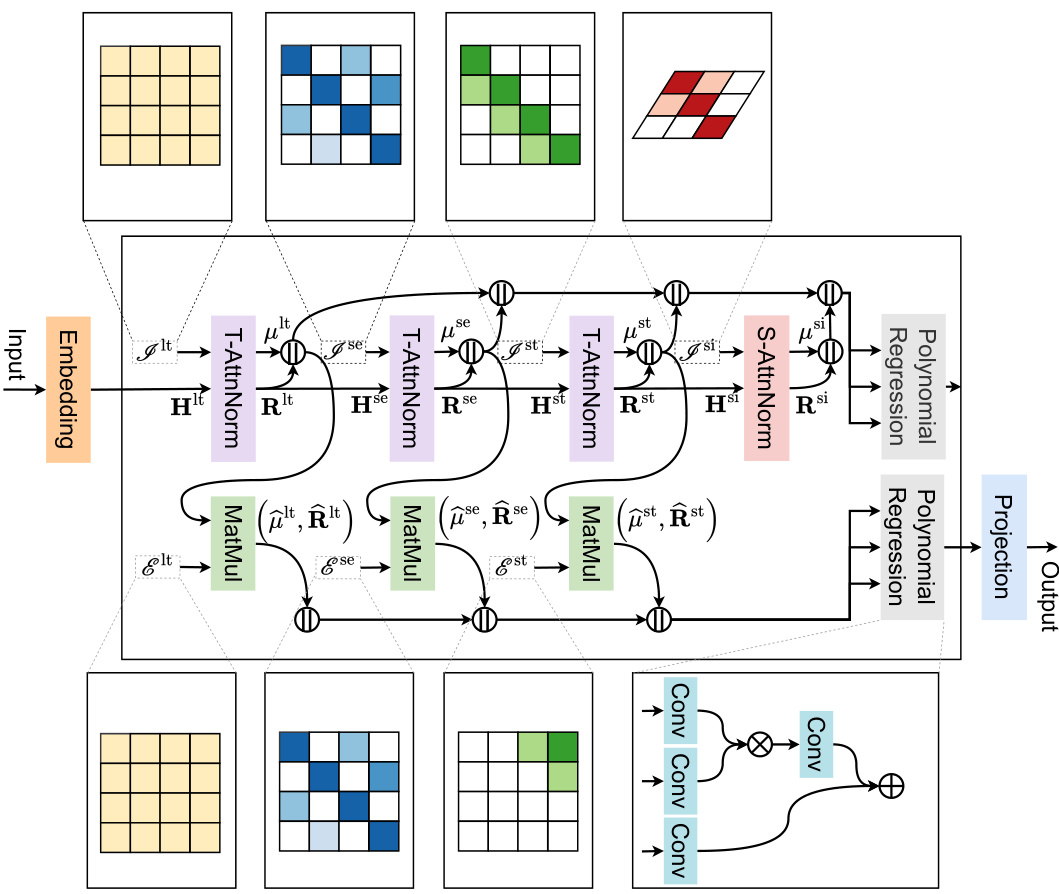
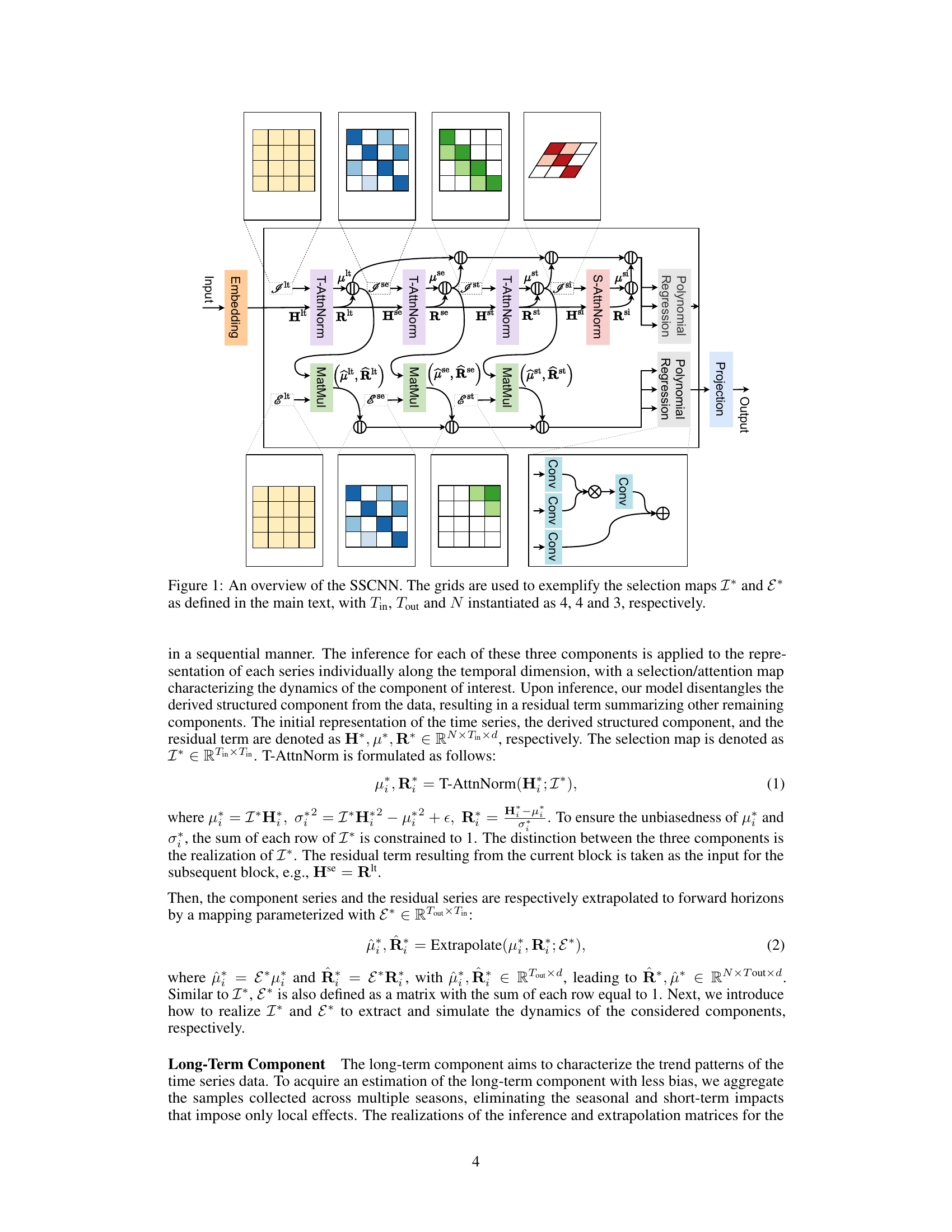
This figure provides a visual representation of the Selective Structured Components-based Neural Network (SSCNN) architecture. It shows the flow of data through the different components of the model: embedding, inference of long-term, seasonal, and short-term components (using T-AttnNorm and selection maps I*), inference of spatial components (using S-AttnNorm and selection maps I*), extrapolation of components (using Extrapolate and selection maps E*), and finally component fusion using polynomial regression. The grids illustrate the selection maps, showing how the model selectively focuses on specific parts of the input sequence for each component.

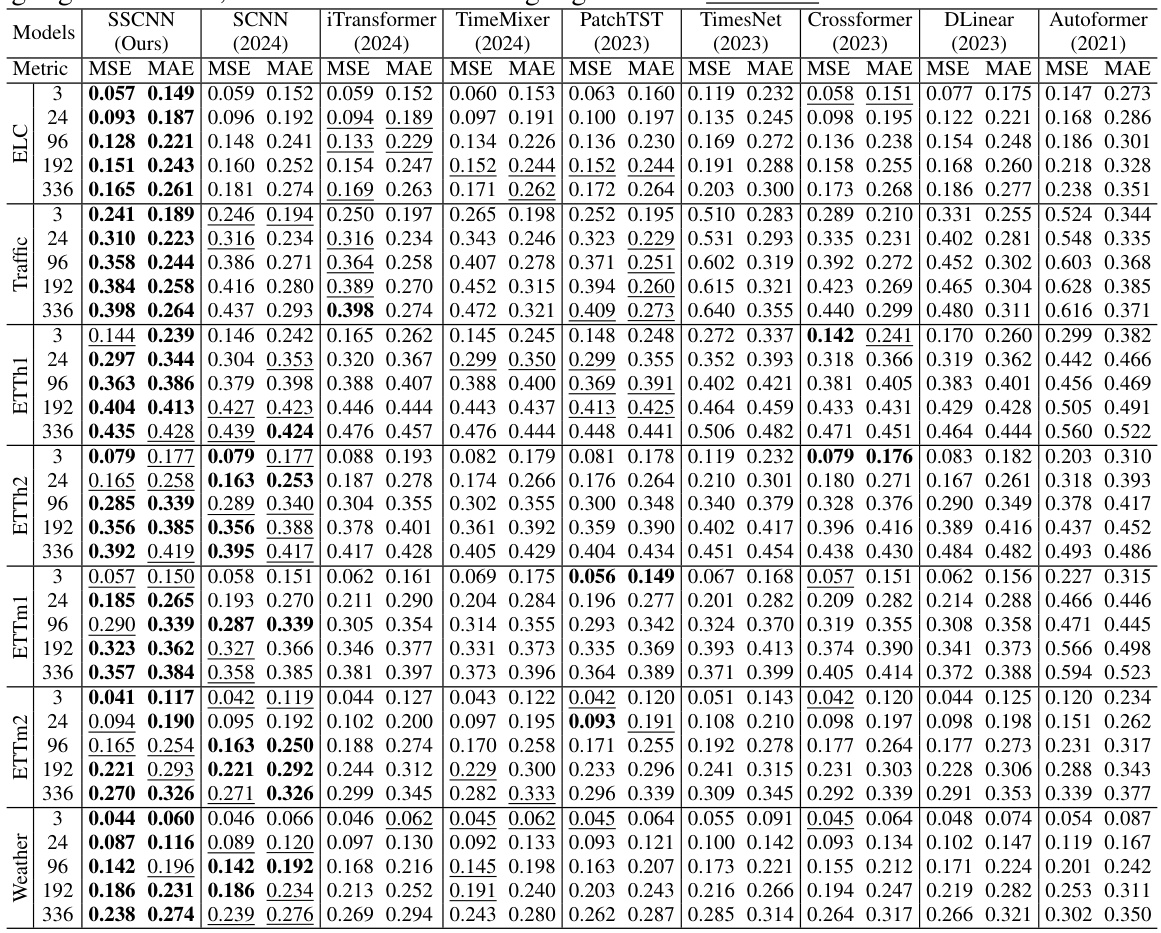
This table presents the mean squared error (MSE) and mean absolute error (MAE) for seven real-world datasets using various long-term forecasting models. The models include SSCNN (the proposed model), DLinear, Autoformer, SCNN, iTransformer, TimeMixer, PatchTST, TimesNet, and Crossformer. The best and second-best results for each dataset and metric are highlighted for comparison.

In-depth insights

#

LTSF Decomposition

#

Long-term time series forecasting (LTSF) presents unique challenges due to the extensive length of input sequences. Traditional approaches often address this by increasing model complexity, leading to millions of parameters. LTSF decomposition offers a compelling alternative, aiming to achieve superior performance with far fewer parameters. This method focuses on breaking down the time series into constituent components (e.g., trend, seasonality, short-term fluctuations) before modeling each component separately. The key advantage lies in reducing model redundancy. Instead of using a monolithic model to capture all aspects, decomposition allows for specialized models, each optimized for a specific component. This leads to more robust and efficient learning and greatly reduces the number of parameters needed. While decomposition methods have shown promise, further research into selecting and effectively combining decomposed components is crucial for achieving optimal results. Combining this with advanced architectures may further boost accuracy and efficiency.

SSCNN Architecture

#

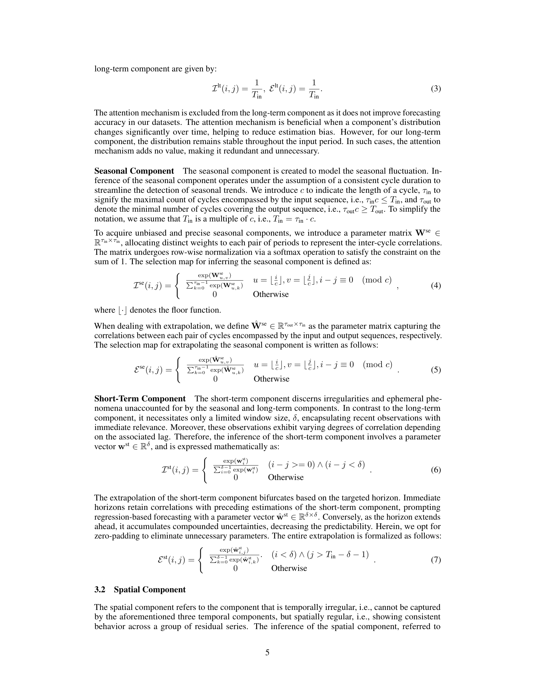
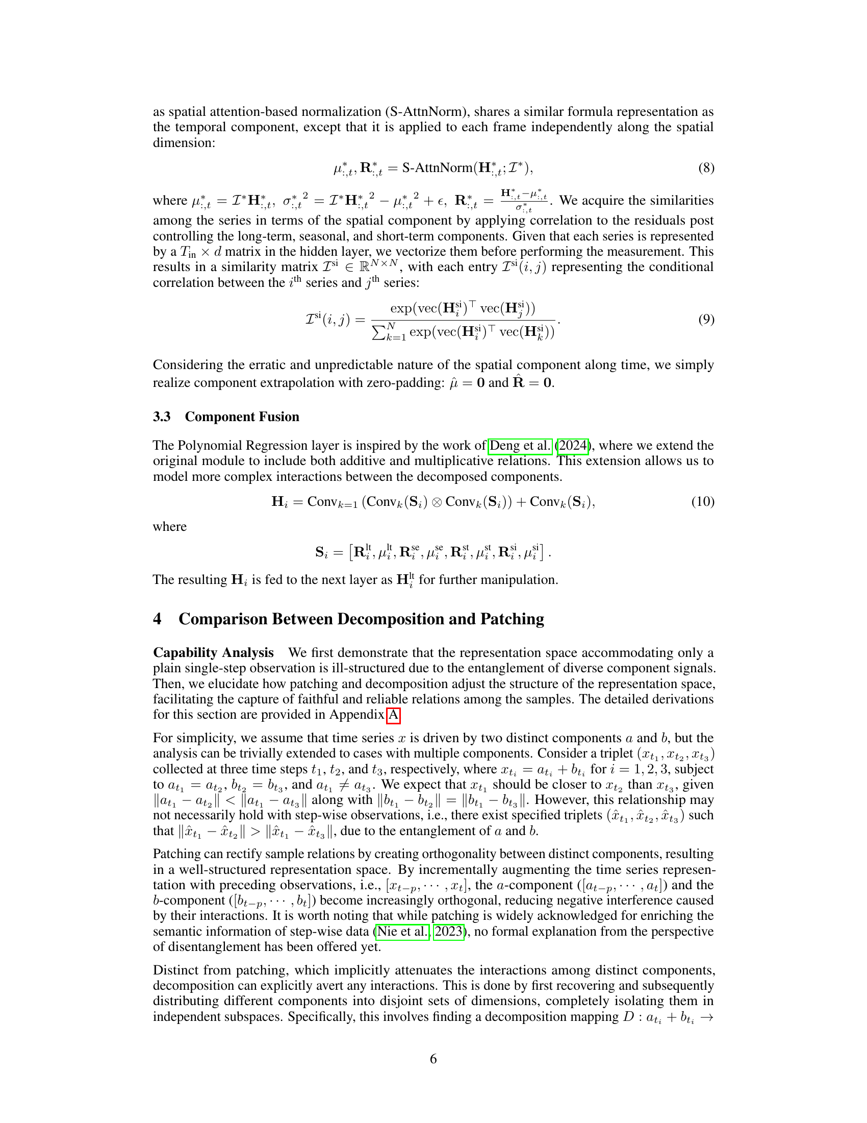
The SSCNN architecture is a novel approach to long-term time series forecasting that leverages selective structured component decomposition to achieve both parsimony and high accuracy. Unlike methods relying on massive parameter scaling, SSCNN decomposes the time series into interpretable components (long-term trend, seasonality, short-term fluctuations, and spatial correlations). A crucial aspect is the selection mechanism that filters out irrelevant information within each component. The inference and extrapolation processes for each component involve unique attention mechanisms tailored to their dynamic characteristics. This design not only reduces the model’s dimensionality significantly but also ensures that the model focuses on the essential features, improving its generalization capabilities. Finally, polynomial regression fuses the components, capturing complex interdependencies to deliver accurate long-term forecasts. The overall architecture demonstrates a shift from massive model scaling towards efficient and accurate forecasting with substantially fewer parameters, making SSCNN highly effective and computationally efficient.

Parsimony vs. Patching

#

The core of the ‘Parsimony vs. Patching’ discussion lies in contrasting the model complexity and efficiency. Patching methods, while effective in capturing long-range dependencies, often lead to excessive model size and computational cost due to their reliance on high-dimensional latent spaces. In contrast, parsimonious approaches like decomposition prioritize maintaining temporal and spatial regularities using fewer parameters. The central argument is that by selectively decomposing a time series into structured components, models can achieve superior accuracy with significantly reduced complexity and computational burden, thereby achieving both capability and parsimony. This trade-off emphasizes that model size is not directly correlated with performance, and that focusing on efficient representation of inherent data structures is crucial for long-term forecasting.

Hyperparameter Analysis

#

A thoughtful hyperparameter analysis is crucial for assessing a model’s robustness and generalizability. It should explore how variations in key hyperparameters influence performance across different metrics and datasets. Detailed visualizations are important to see trends and interactions. For example, instead of simply reporting the best performing hyperparameters, it is beneficial to show how changes affect multiple metrics (e.g., accuracy vs. computational cost) over various datasets, helping to understand tradeoffs. The analysis should also comment on the sensitivity of the model to different hyperparameters. Some might have a significant impact, whereas others might only affect the model marginally. Finally, a rigorous methodology is vital for ensuring the reliability of results. Techniques like cross-validation and statistical significance tests must be utilized. By presenting a detailed hyperparameter analysis, we can gain better insights into the model and its behavior, making informed decisions about its use in diverse applications.

Future of LTSF

#

The future of Long-Term Time Series Forecasting (LTSF) hinges on addressing current limitations. Parsimony is key; excessively complex models with millions of parameters offer diminishing returns. Future research should focus on more efficient architectures that leverage decomposition techniques and selection mechanisms, as demonstrated in the paper’s SSCNN model. Improved analytical understanding of feature decomposition’s relationship to patching is needed, along with exploring new ways to leverage domain-specific characteristics for more accurate and robust forecasts. Handling irregular time series data and incorporating probabilistic approaches will also be critical for improved real-world applicability. Furthermore, the ethical implications of LTSF, including potential misuse and biases, require careful consideration in model development and deployment. Ultimately, the successful future of LTSF rests on balancing capability with efficiency and responsibility.

More visual insights

#

More on figures

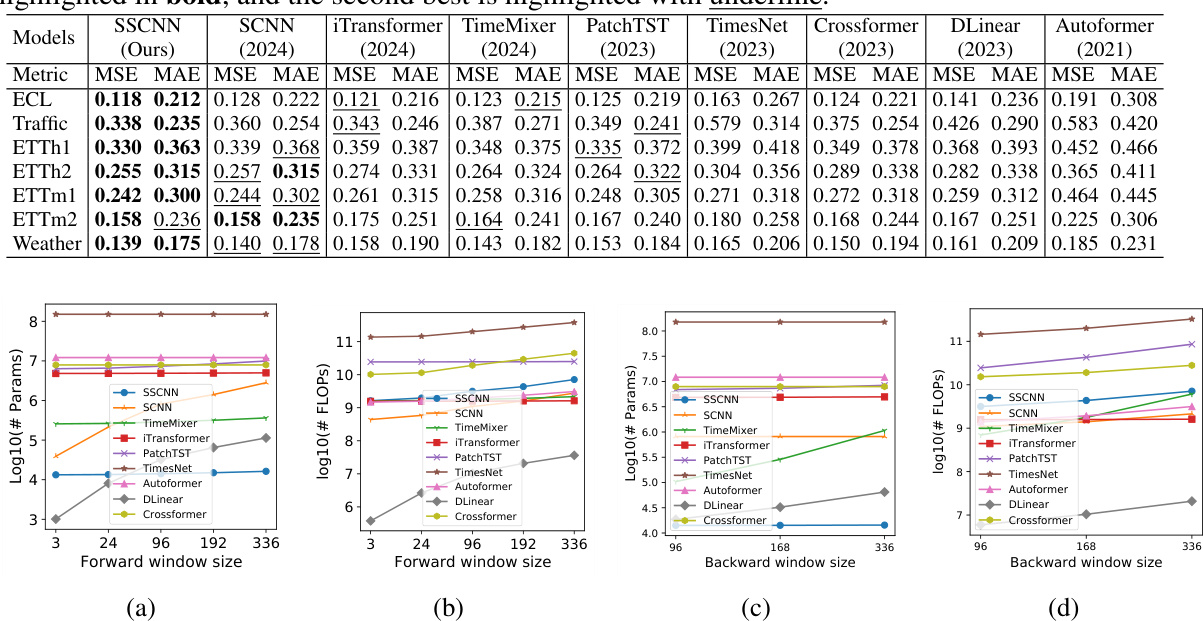
This figure shows the parameter scale and computational cost (measured in FLOPs) of SSCNN and other state-of-the-art models across varying forward and backward window sizes for the ECL dataset. It demonstrates SSCNN’s efficiency in terms of both parameters and computation, especially when compared to other Transformer-based models. The plots visualize the relationship between window size and model complexity, highlighting the parsimonious nature of SSCNN.

This figure shows the impact of the backward window size on the MSE of different models for four different settings. The settings vary the dataset (ECL or ETTh2) and the forward window size (24 or 336). In general, increasing the backward window size improves the MSE. However, the improvement is more significant for certain settings than for others. For example, in (a) ECL Tout=24, increasing the backward window size from 96 to 336 results in a significant drop in MSE. However, in (d) ETTh2 Tout=336, the improvement is marginal.

This figure displays the sensitivity analysis of five hyperparameters (number of layers, hidden dimension, kernel size, cycle length, and short-term span) on the performance of the SSCNN model, using the ECL and Traffic datasets. Each subplot shows how changes in a single hyperparameter affect the model’s performance, while holding the others constant. This analysis aims to identify the most influential hyperparameters for tuning the model’s accuracy.

This ablation study analyzes the impact of each component (long-term, seasonal, short-term, spatial) and attention mechanisms within the SSCNN model on two datasets (ECL and Traffic). Removing components or attention mechanisms individually shows significant performance degradation, highlighting their importance for accurate forecasting. The use of a fully-connected network (FCN) shows no improvement and may be redundant.

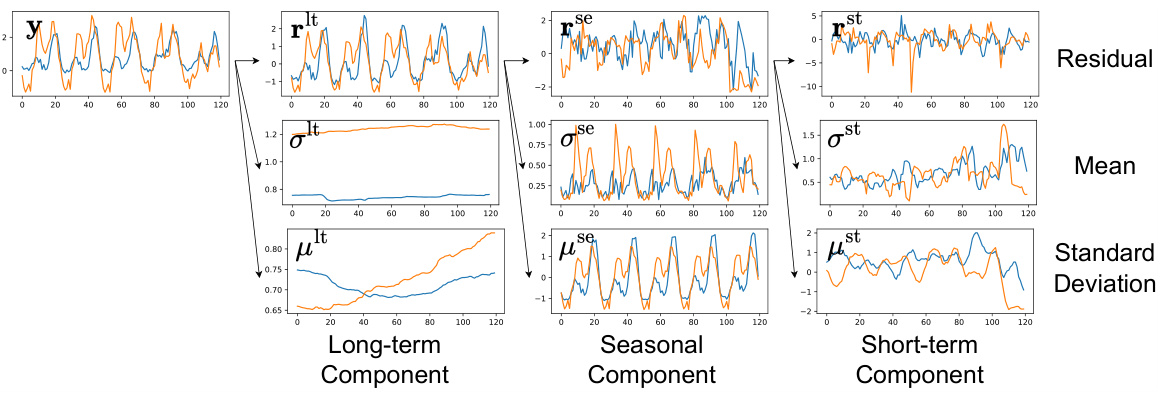
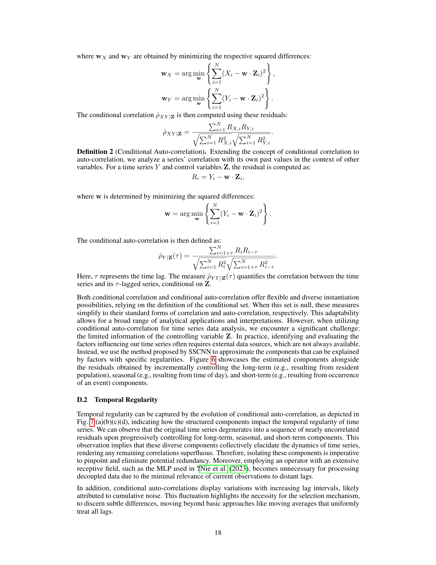
This figure visualizes the decomposition of a time series into its structured components (long-term, seasonal, and short-term) and a residual component. For each component, the figure shows the original time series (blue), the extracted component (orange), the mean, and the standard deviation of the component. The decomposition process helps in isolating the different patterns that contribute to the overall time series.

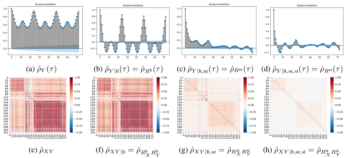
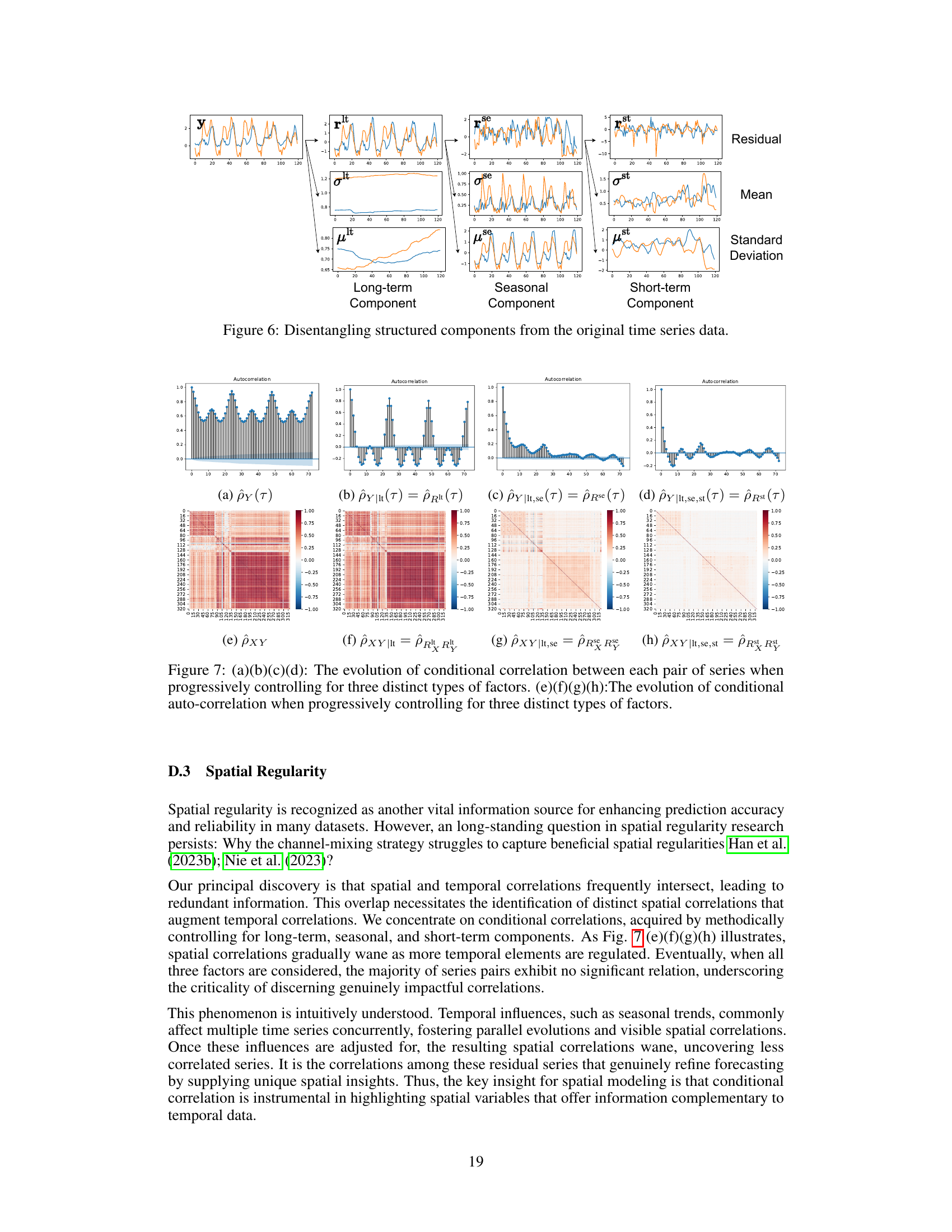
This figure visualizes how conditional correlations and autocorrelations change as the long-term, seasonal, and short-term components are progressively controlled for. The top row shows the autocorrelations for the original time series and after removing each component. The bottom row shows the corresponding conditional correlation matrices. This illustrates how removing structured components reveals the remaining, less correlated components.

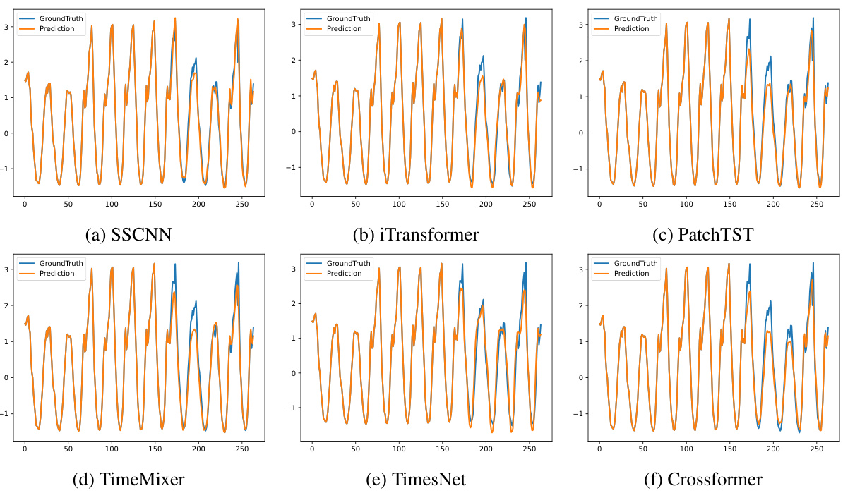
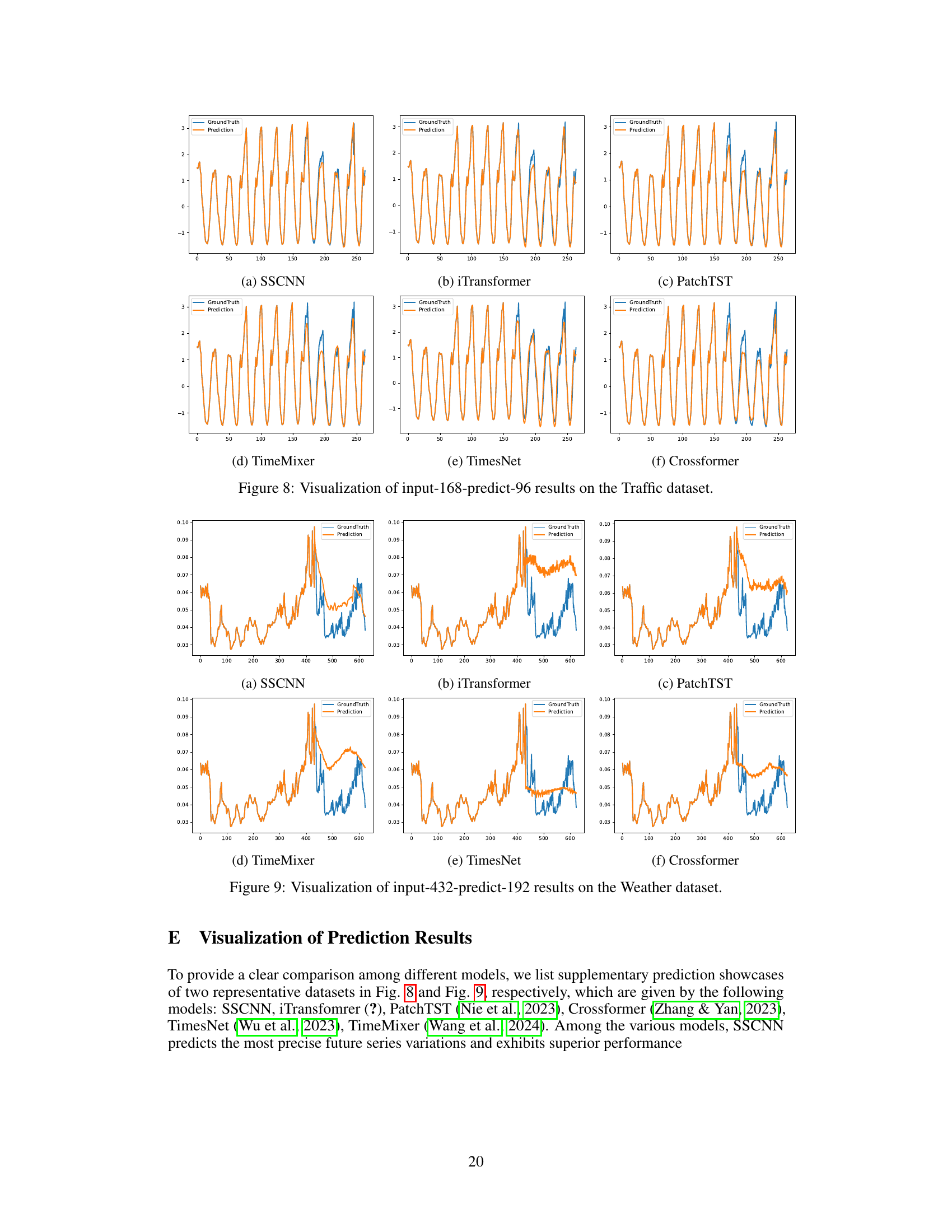
This figure visualizes the prediction results of six different time series forecasting models (SSCNN, iTransformer, PatchTST, TimeMixer, TimesNet, and Crossformer) on the Traffic dataset. The input sequence length was 168 time steps, and the prediction horizon was 96 time steps. The figure allows a visual comparison of the accuracy and patterns captured by each model in comparison to the ground truth.

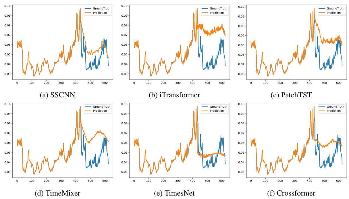
This figure visualizes the performance of six different time series forecasting models (SSCNN, iTransformer, PatchTST, TimeMixer, TimesNet, and Crossformer) on the Traffic dataset. Each model’s prediction is plotted against the ground truth for a sequence length of 168 inputs and 96 predictions. This allows for a direct visual comparison of the accuracy and quality of the different forecasting methods. The visual comparison allows for a quick understanding of each model’s ability to capture the trends and patterns within the Traffic dataset.

Full paper

#