↗ OpenReview ↗ NeurIPS Proc. ↗ Chat
TL;DR#
Current machine learning models for weather forecasting primarily focus on deterministic predictions, neglecting the inherent uncertainties within the chaotic weather system. This limitation restricts the models’ reliability and ability to effectively convey the uncertainty associated with the forecasts. Accurately representing forecast uncertainty is crucial for diverse applications.
To address these challenges, the paper introduces Graph-EFM, a probabilistic forecasting model that uses a hierarchical graph neural network architecture. This method enhances the efficiency of ensemble forecasting by enabling the generation of large ensembles using a single forward pass per time step. Through experiments on global and limited-area datasets, Graph-EFM demonstrates superior performance in capturing forecast uncertainty and achieving equivalent or lower forecast errors when compared to deterministic methods. The hierarchical structure of Graph-EFM encourages spatially coherent forecasts, further improving prediction quality. This model represents a significant advancement in probabilistic weather forecasting, offering improved decision-making capabilities for various sectors dependent on accurate and reliable weather information.
Key Takeaways#
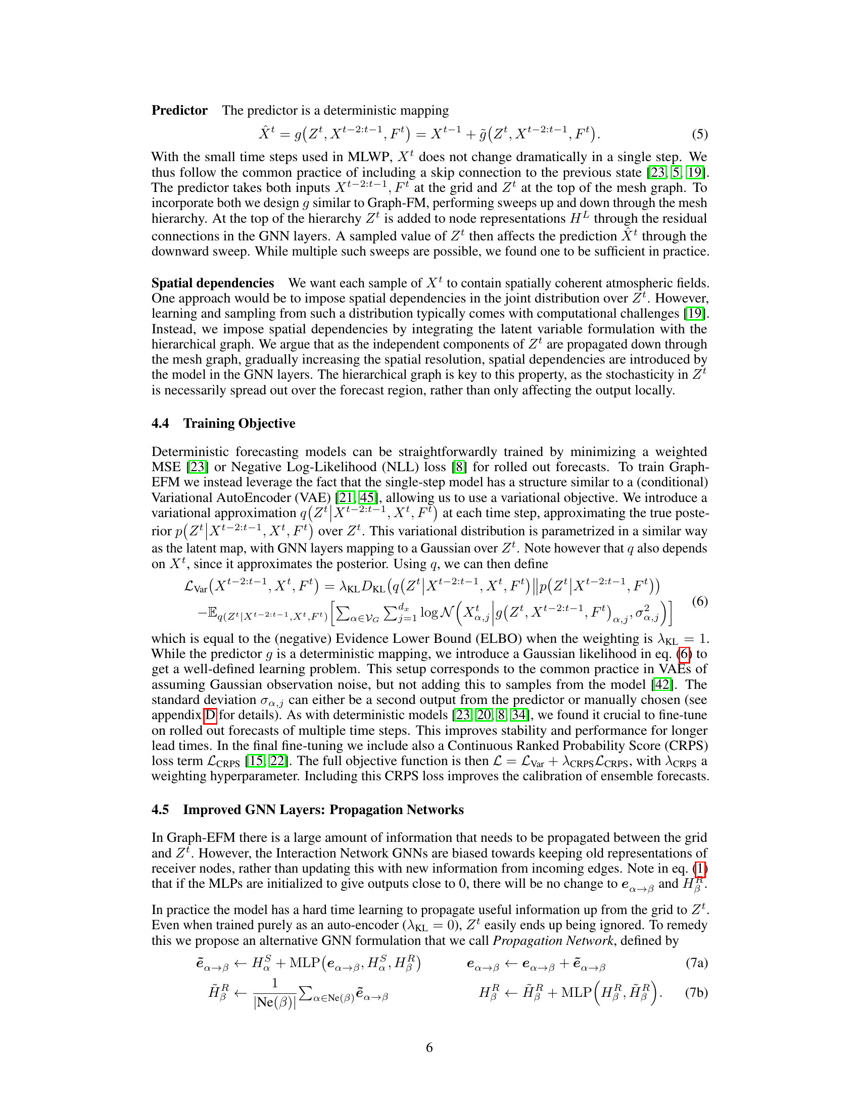
Why does it matter?#
This paper is crucial for researchers in machine learning and weather forecasting. It introduces a novel probabilistic model that efficiently generates large ensembles, overcoming a major limitation of current methods. This significantly improves forecast accuracy and uncertainty quantification, directly impacting various sectors dependent on reliable weather prediction. The hierarchical graph neural network approach is also highly relevant to other spatial prediction problems, opening new research avenues in graph-based machine learning.
Visual Insights#

This figure shows a schematic overview of the Graph-EFM model. It illustrates how the model processes data at different levels of a hierarchical graph to produce probabilistic forecasts. The input data includes past weather states, forcing data, and boundary conditions (in the limited-area case). This data is fed into a series of graph neural network layers, and the latent variable Zt is sampled at the top of the hierarchy. The prediction for the next time step is made by processing data from lower levels in a way similar to Graph-FM, using residual connections to incorporate the latent variable. The process is repeated to make a prediction for each time step in the forecasting horizon.
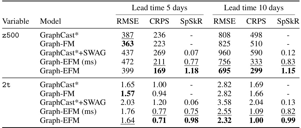
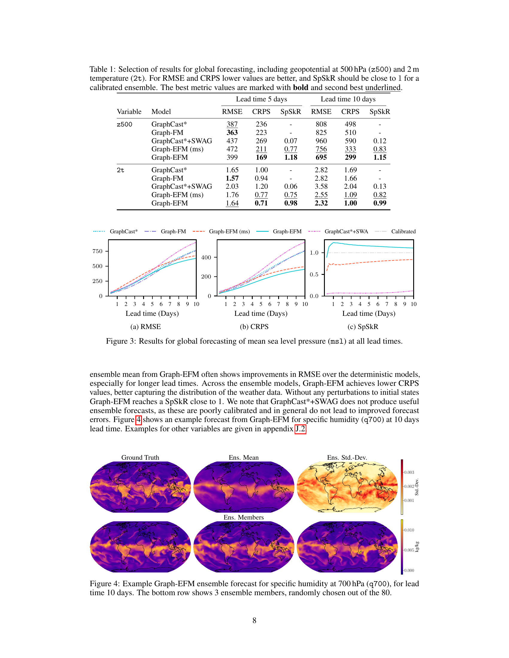
This table presents a selection of the results for global forecasting experiments at lead times of 5 and 10 days. It shows the RMSE, CRPS, and SpSkR values for different models: GraphCast*, Graph-FM, GraphCast*+SWAG, Graph-EFM (ms), and Graph-EFM. Lower values for RMSE and CRPS indicate better performance, while a SpSkR value close to 1 signifies well-calibrated uncertainty. The best and second-best results for each metric are highlighted.
In-depth insights#
Graph-EFM Model#
The Graph-EFM model, a probabilistic weather forecasting model, stands out for its efficient ensemble generation, achieved through a single forward pass per time step. This efficiency is enabled by its hierarchical graph neural network (GNN) architecture, which facilitates the efficient sampling of spatially coherent forecasts. The model combines a flexible latent-variable formulation with a graph-based forecasting framework, allowing it to capture forecast uncertainty effectively. Unlike methods relying on ad-hoc perturbations, Graph-EFM directly models the full distribution, resulting in better calibrated ensembles. Its application to both global and limited-area forecasting demonstrates its adaptability and potential for high-resolution prediction, offering a promising advance in probabilistic weather forecasting.
Hierarchical GNNs#
The concept of “Hierarchical GNNs” suggests a powerful extension to standard graph neural networks (GNNs). By introducing a hierarchy, the model can efficiently capture multi-scale features present in complex data. This is especially relevant for applications where information exists at various levels of granularity, such as in weather forecasting where global patterns influence local dynamics. A hierarchical architecture enables the network to learn representations at different scales. This is crucial, as lower levels would focus on fine-grained details while upper levels would encapsulate broader trends. The hierarchical approach enables spatially coherent processing and also contributes to efficient ensemble generation, which is essential for probabilistic forecasting. It is worth noting that the specific implementation details, such as the graph construction and message-passing mechanisms within each hierarchical level, are key determinants of the model’s overall performance and accuracy. Careful design of the hierarchical structure is therefore paramount to fully exploit its potential advantages.
Ensemble Forecasting#
Ensemble forecasting, a crucial aspect of probabilistic weather prediction, tackles the inherent uncertainty in weather systems by generating multiple forecasts, each representing a plausible future weather scenario. Instead of providing a single deterministic prediction, ensemble methods offer a probability distribution of potential outcomes, allowing for a more comprehensive understanding of forecast uncertainty. This is particularly valuable for extreme weather events and crucial decisions like infrastructure planning and disaster preparedness. The success of ensemble forecasting hinges on several factors: the accuracy of each individual forecast, the diversity of the ensemble members, and the calibration of the forecast uncertainty. Computational costs and efficient sampling techniques are key considerations for developing large-scale ensemble forecasting systems. Machine learning approaches offer innovative ways to address these challenges, enabling efficient generation of large ensembles at high spatial resolutions—an area of active research and development.
Uncertainty Modeling#
In the realm of probabilistic weather forecasting, uncertainty modeling is paramount. The chaotic nature of atmospheric systems introduces inherent unpredictability, making deterministic forecasts insufficient. Effective uncertainty modeling captures this variability, not just by predicting the most likely outcome, but also by quantifying the range of possible future weather states. This is typically achieved through ensemble forecasting, where multiple forecasts are generated and their distribution is analyzed. Methods for uncertainty modeling often involve probabilistic models that explicitly represent the uncertainty using probability distributions, such as Bayesian networks or Gaussian processes. These models allow for quantifying the confidence associated with each forecast, thereby enhancing the value and reliability of weather predictions for decision-making.
Future of MLWP#
The future of Machine Learning-based Weather Prediction (MLWP) is bright, but faces challenges. Improved data quality and quantity, particularly high-resolution observations from diverse sources, will be crucial. More sophisticated model architectures, potentially incorporating hybrid physical-MLWP approaches, will enhance accuracy and efficiency. Addressing uncertainty through probabilistic methods remains paramount; research needs to focus on producing well-calibrated and diverse ensembles effectively. Further investigation is needed to determine how best to leverage explainability techniques to build confidence in MLWP forecasts and understand their limitations, especially for extreme weather events. Ultimately, the future of MLWP depends on addressing these challenges to make weather predictions faster, more accurate, and more readily usable for diverse applications.
More visual insights#
More on figures

This figure shows the graphical model representation of the single-step probabilistic weather forecasting model proposed by the authors. The model introduces a latent variable Zt, representing the uncertainty at time step t, which influences the prediction Xt of the weather state at time t. The model assumes a second-order Markov property, indicating that Xt depends on Xt-1, Xt-2, and Zt. The figure visually depicts these dependencies and the conditional probability distribution that the model aims to capture.

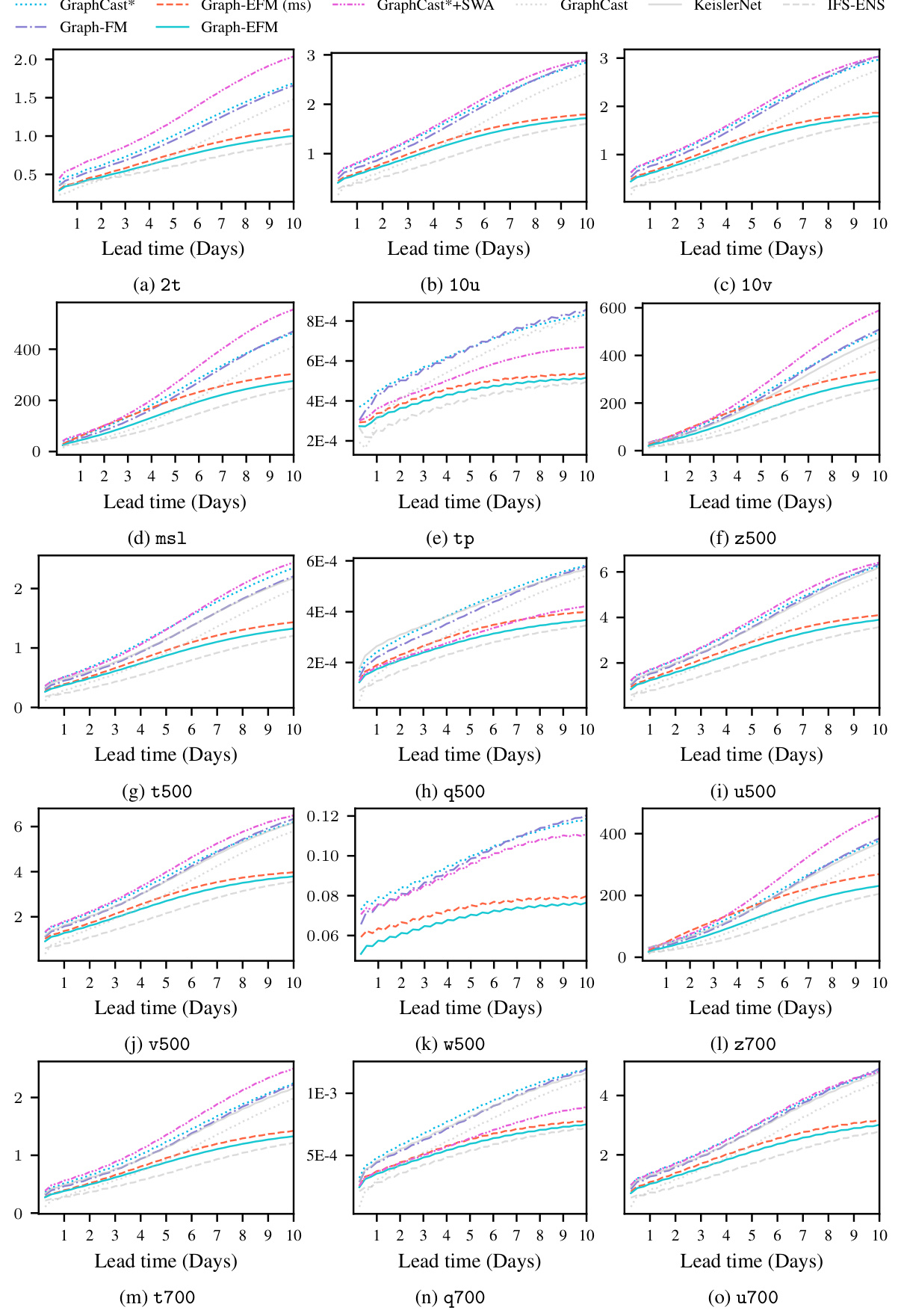
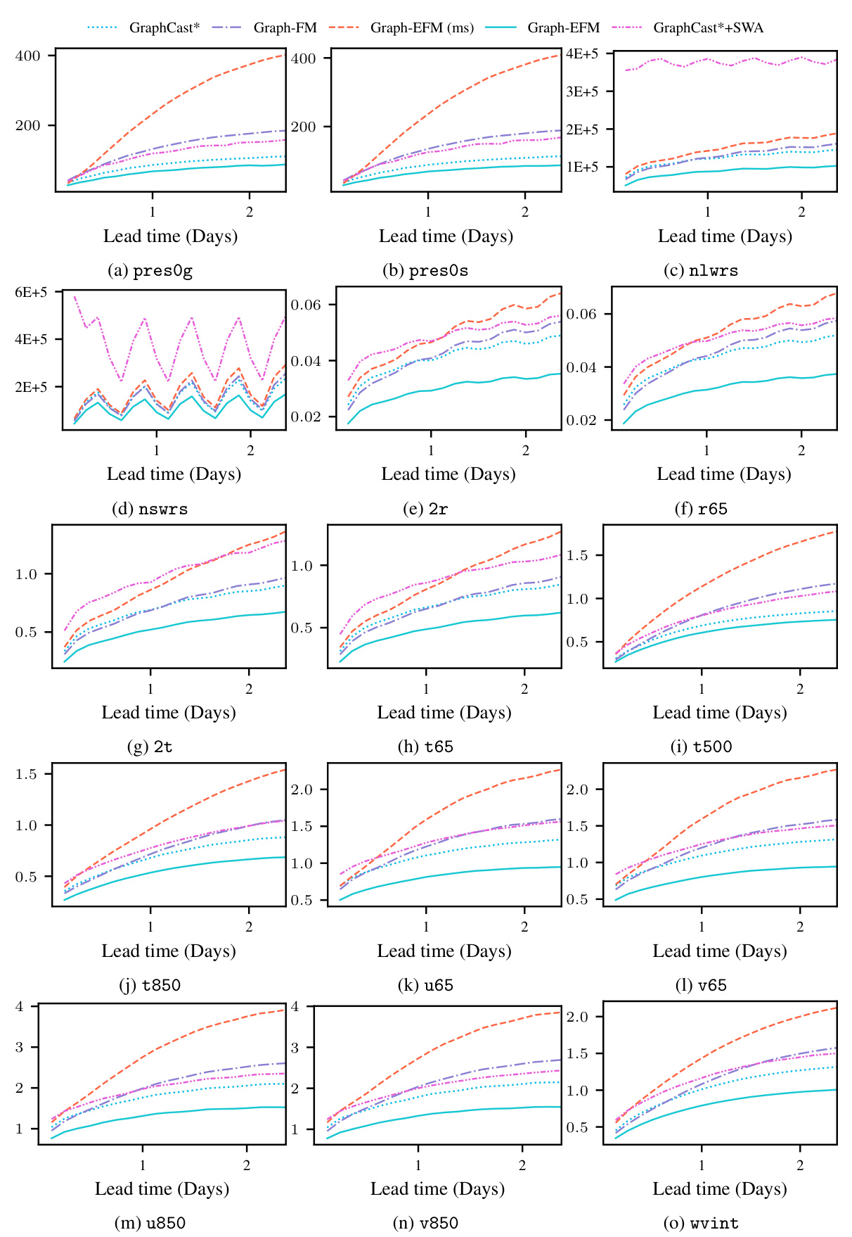
The figure shows the RMSE, CRPS and SpSkR for mean sea level pressure forecasts using GraphCast*, Graph-FM, GraphCast*+SWAG, Graph-EFM (ms) and Graph-EFM. The results are shown for lead times of up to 10 days. The plot shows that Graph-EFM achieves lower CRPS values than the other methods, indicating better probabilistic forecasting performance. Graph-EFM also shows good calibration (SpSkR close to 1), indicating that the ensemble spread accurately reflects the forecast uncertainty. GraphCast*+SWAG does not produce useful ensemble forecasts as they are poorly calibrated and do not lead to improved forecast errors.
The figure compares the forecasts of three global weather models (GraphCast*, Graph-FM, and Graph-EFM) with ground truth data at a 10-day lead time. The models are evaluated on three key variables: the u-component of wind at 10 meters (10u), specific humidity at 700 hPa (q700), and geopotential at 500 hPa (z500). The probabilistic models (Graph-EFM) show sampled ensemble members, illustrating the uncertainty inherent in the forecasts, while the deterministic models provide a single forecast value.

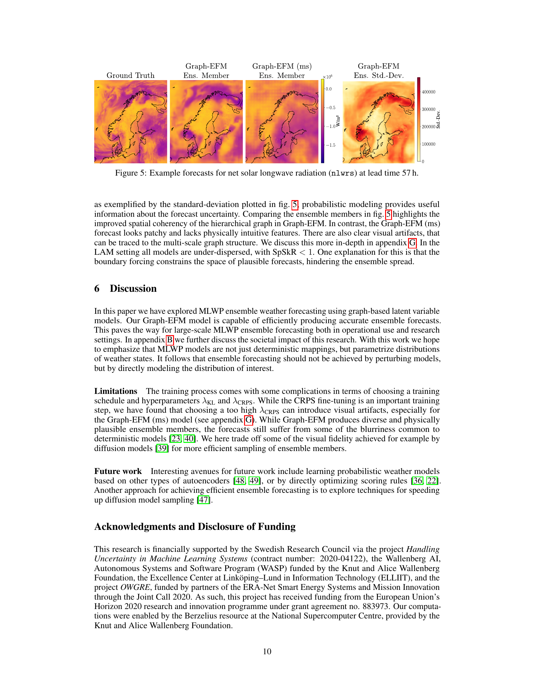
This figure compares example forecasts for net solar longwave radiation (nlwrs) at a lead time of 57 hours. It showcases the ground truth, ensemble mean and standard deviation from Graph-EFM, and an ensemble member forecast from Graph-EFM (ms) and Graph-EFM. The visualization highlights the differences in spatial coherency between the models. Graph-EFM using the hierarchical graph shows improved spatial coherence compared to the Graph-EFM (ms) model using the multi-scale graph, demonstrating a key benefit of the hierarchical approach in representing spatially continuous atmospheric fields.

This figure shows a schematic overview of the Graph-EFM model, illustrating the flow of information and the hierarchical graph structure used. It depicts the process of generating an ensemble forecast using a latent variable model combined with a hierarchical Graph Neural Network. The model starts with initial states and forcing data, which are mapped to a lower-dimensional latent space. Samples are drawn from this latent space and then used to generate predictions for the next timestep using a deterministic Graph-FM model. This process is repeated for a sequence of time steps, producing a spatially coherent ensemble forecast. The figure highlights both the latent variable modeling aspect and the hierarchical structure of the Graph Neural Network. A separate illustration for global forecasting is available in Appendix C.

This figure shows a schematic overview of the Graph-EFM model, illustrating how the model processes data and generates forecasts. It highlights the use of a hierarchical graph neural network (GNN) and latent variables to capture forecast uncertainty. The example shows the Limited Area Model (LAM) setup, but a similar schematic is provided in the appendix for the global model. The model takes as input the previous weather states, forcing inputs, and potentially boundary conditions (for the LAM case). It uses a hierarchical GNN to process this information, then uses a latent variable to introduce stochasticity to capture uncertainty. Finally, it samples from the latent variable’s distribution and generates the forecast. The residual connection between outputs and previous time steps is shown.

This figure compares forecasts of 10 m wind speeds during Hurricane Laura from different models at various lead times (7 days, 5 days, 3 days, and 1 day before the event). The first column displays ERA5 reanalysis data, while subsequent columns show forecasts from Graph-EFM (including 4 random ensemble members and a best-matching member), GraphCast*, and Graph-FM. The figure highlights the differences in the models’ ability to capture the hurricane’s intensity and location at different timescales and the uncertainty represented by the Graph-EFM ensemble.

This figure compares example forecasts generated by Graph-EFM and Graph-EFM (ms) models trained on the MEPS dataset. The forecasts are for a lead time of 57 hours and highlight the differences in spatial coherence between the two models. Graph-EFM, using a hierarchical graph, produces forecasts that are more spatially coherent, whereas Graph-EFM (ms), using a multi-scale graph, shows patchier and less realistic-looking results.

This figure shows example forecasts from Graph-EFM and Graph-EFM (ms) models trained on MEPS data, showcasing ensemble members’ forecasts for different variables at a lead time of 57 hours. It visually demonstrates the difference in spatial coherence between the hierarchical (Graph-EFM) and multi-scale (Graph-EFM (ms)) graph approaches.

This figure compares the forecasts from four different models for u-component of wind at 850 hPa and 2 m relative humidity at 57 h lead time. It includes the ground truth, GraphCast*, Graph-FM and two versions of Graph-EFM. The Graph-EFM model outputs show sampled ensemble members, highlighting the range of possible forecasts.

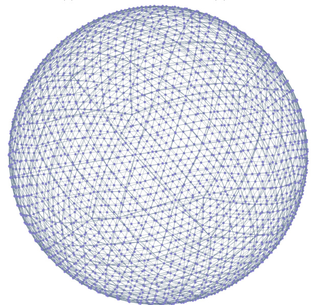
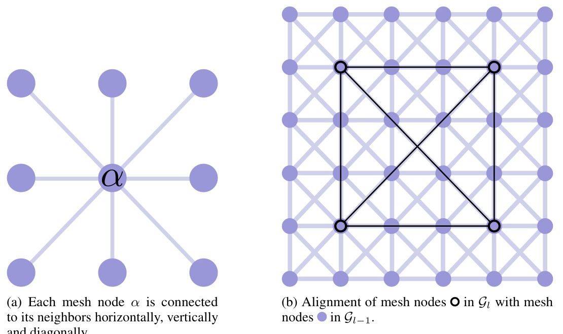
This figure shows different mesh graphs used in the global forecasting experiments described in the paper. Specifically, it visualizes the multi-scale mesh graph (GMS) created by recursively splitting the faces of an icosahedron, and the hierarchical mesh graph used in the Graph-EFM model. The hierarchical graph is composed of several graphs (G1, …, G5), each with varying edge lengths and node connections representing different spatial scales. The inter-level graph (G3,4) illustrates the connections between the different levels of the hierarchy. The visualization is intended to highlight the structural differences between the multi-scale and hierarchical graph approaches. Note that the vertical placement of the nodes is for visualization and doesn’t reflect the actual spatial arrangement.

This figure shows different mesh graphs used in the global forecasting experiments described in the paper. Panel (a) through (d) show the multi-scale mesh graphs G1 to G4 created by recursively splitting the faces of an icosahedron. Panel (e) shows the final multi-scale mesh graph GMS, which includes all nodes from G1, but connects them using edges from all levels (G1 to G4). Panel (f) shows the hierarchical mesh graph used by the Graph-EFM model, which is based on G4 to G1 but adds explicit connections between the levels. Panel (g) shows an example of the inter-level graphs used to connect the different levels in the hierarchy, in this case between G3 and G4.

This figure shows different mesh graphs used in the global weather forecasting experiment. It illustrates the construction of multi-scale and hierarchical mesh graphs. The multi-scale graph (e) is created by recursively splitting the faces of an icosahedron and merging the resulting graphs. The hierarchical graph (f) uses a sequence of graphs at different levels, connecting them through edges between levels. (g) shows a zoom on an inter-level graph illustrating the connections between different levels in the hierarchy. The vertical positioning of the nodes in the figure is solely for illustrative purposes; the actual graph structure is represented on a 2D sphere.
This figure shows different mesh graphs used in the global weather forecasting experiment. Panel (a) through (d) show the different levels of the hierarchical mesh graph, from coarser (a) to finer (d) resolutions. (e) shows the multi-scale mesh graph, which combines all levels to capture multiple spatial scales. Panel (f) shows the hierarchical mesh graph used in the Graph-EFM model. (g) illustrates the connections between levels l and l+1 in the hierarchical graph. The vertical positioning is for visualization and does not reflect the true structure.

This figure shows different mesh graphs used in the global forecasting experiments. It includes (a) to (d) individual mesh graphs at different levels of resolution (G1 to G4) from the finest to the coarsest. Then (e) shows the multi-scale mesh graph (GMS) combining all levels, while (f) illustrates the hierarchical mesh graph used in the Graph-EFM model. Finally (g) shows an example of an inter-level graph (G3,4) connecting nodes at adjacent levels in the hierarchy.

This figure shows different mesh graphs used in the global weather forecasting experiment. It illustrates the multi-scale mesh graph (GMS), constructed by recursively subdividing the faces of an icosahedron, and the hierarchical mesh graph used in the Graph-EFM model. The hierarchical graph comprises multiple levels of graphs (G1 to G4 in this example), with connections between adjacent levels, creating a multi-resolution representation of the globe. The image also shows a single level of the inter-level graph, demonstrating the connections between different levels. Note that the vertical positioning of nodes is merely for visual clarity and does not reflect the actual 3D representation.
This figure shows a schematic overview of the Graph-EFM model, illustrating the flow of data and information through the model’s components. It highlights the use of hierarchical graphs, latent variables, and a combination of deterministic and probabilistic components. The left side depicts the input data, including the previous weather states and forcing inputs. The middle shows the Graph-FM model used for prediction, employing a graph neural network processing on a hierarchical graph. The right illustrates how latent variables are sampled, and a residual connection is used to generate the ensemble forecasts. The figure also provides a specific example using a limited area model, with a reference to a similar figure in the appendix showing the model for global forecasting.

This figure shows different mesh graphs used in the global forecasting experiment. It includes subfigures (a) to (d) showing the multi-scale mesh graphs G1 to G4 which are successively created by splitting the faces of an icosahedron. Subfigure (e) shows the multi-scale mesh graph GMS constructed by merging all the nodes from G1-G4 but using edges from all levels. Subfigure (f) shows the hierarchical mesh graph created by using G4-G1 as different layers in the hierarchy with additional inter-level edges and (g) shows one of the inter-level graphs G3,4. The graphs are visualized in 3D for better understanding but the vertical positioning is only for visualization purposes.
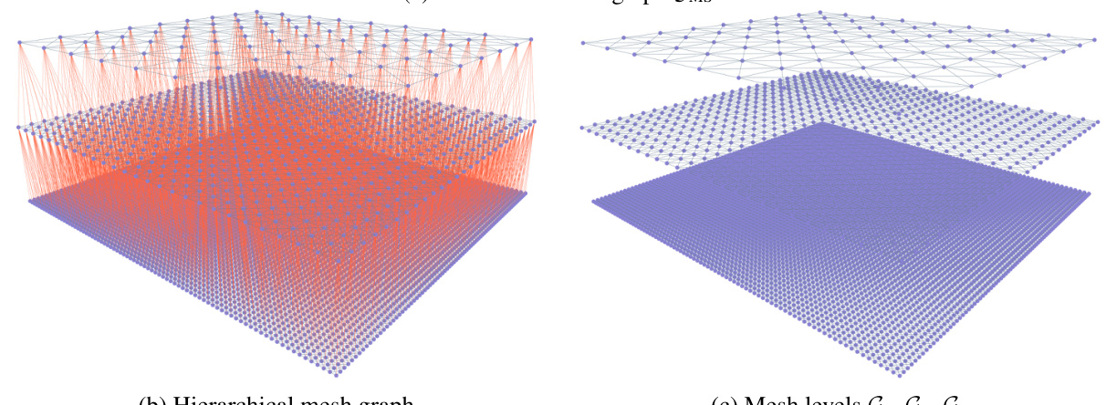
This figure shows different mesh graphs used in the global forecasting experiment. Panel (a) through (d) illustrate the multi-scale mesh graphs created by recursively splitting faces of an icosahedron, resulting in graphs G1 through G4. Panel (e) shows the multi-scale mesh graph GMS created by merging the nodes from G1 while connecting them with edges from all four graphs. This approach allows the model to capture both local and long-range dependencies. Panel (f) displays the hierarchical mesh graph used in the proposed Graph-EFM model, showing the four levels G1 through G4. The hierarchical structure facilitates efficient information propagation at multiple spatial scales. Finally, panel (g) illustrates an example inter-level graph connecting levels G3 and G4, highlighting the connections between different levels of the hierarchy.

This figure shows a schematic overview of the Graph-EFM model, illustrating the flow of data and the hierarchical graph structure used for a limited area model. The initial weather states (Xt−2:t−1) and forcing data (Ft) are input to the model. The model uses a latent variable (Zt) to represent the uncertainty in the forecast. Samples of Zt are drawn from a latent map p(Zt|Xt−2:t−1, Ft), which is a neural network that operates on a hierarchical graph (G1, …,GL). The sampled Zt is then passed through a deterministic forecasting model (Graph-FM) to generate the forecast (Xt). A residual connection is also utilized. The figure also includes examples of the types of graphs used for the limited area model.

This figure shows a schematic overview of the Graph-EFM model for limited area weather forecasting. It illustrates the model’s workflow, beginning with input data (previous weather states Xt-2:t-1, boundary conditions Bt, and forcing Ft), proceeding through a hierarchical graph neural network (GNN), and culminating in an output of the predicted weather state Xt. The hierarchical graph structure is highlighted, showing how different levels of the graph capture different spatial scales of the weather system. A key element is the sampling of the latent variable Zt, which introduces uncertainty into the forecast. The figure also provides examples of the data and graph structures used in the model.
This figure shows a schematic overview of the Graph-EFM model. It illustrates how the model processes data from a limited area using hierarchical graphs. The initial states (Xt-2:t-1) and forcing inputs (Ft) are passed through a sequence of graph neural network (GNN) layers, which are organized hierarchically. Each level of the hierarchy captures a different spatial scale, with finer details added as the information is propagated down through the levels. A latent variable (Zt) is introduced to capture forecast uncertainty, which is then sampled to generate multiple ensemble members. Each ensemble member is a possible forecast scenario. The figure also includes a comparison with the global setting, which is detailed in Appendix C.

This figure shows a schematic overview of the Graph-EFM model, illustrating the flow of data through the model. It shows the input data (Xt-2:t-1, Ft, Bt), the hierarchical graph structure used (G1, G2, G3), the latent variable (Zt) and its sampling process, the deterministic predictor (Graph-FM), and the final output (Xt). The example is specifically for a limited area model, while a global model equivalent is presented in Appendix C.
This figure shows a schematic overview of the Graph-EFM model. The model takes as input past weather states (Xt-2:t-1), forcing data (Ft), and for the limited area model, boundary conditions (Bt). These inputs are fed into a latent map that uses a Graph Neural Network (GNN) to generate a latent variable (Zt) representing the uncertainty in the forecast. The latent variable Zt, along with the input data, is then passed through a Graph-FM (Graph-based Forecasting Model) component, which uses a hierarchical GNN to generate a prediction for the current weather state (Xt). Residual connections are shown, indicating that the model uses past weather state information to create the next step. A limited area model and its specific graphs are displayed.

This figure shows example forecasts of 10m wind speeds during Hurricane Laura using ERA5 and different models for the period of 2020-08-27T12 UTC. The first column shows the ground truth of the wind speed from ERA5. The remaining columns show the forecasts from different models initialized at different times before the event. This demonstrates that Graph-EFM provides a good estimate of wind speeds at different lead times and also demonstrates the added value of ensemble forecasts.

This figure shows a schematic overview of the Graph-EFM model. It illustrates the flow of data through the model’s different components, including the input data, latent variable Zt, and the hierarchical graph structure. It highlights the use of Graph-FM as a deterministic sub-model within Graph-EFM, the residual connections, and the sampling process for ensemble generation. The figure also shows an example using a Limited Area Model, with the corresponding overview for the global setting available in Appendix C, Figure 6.

This figure shows a schematic overview of the Graph-EFM model. It illustrates the data flow and the structure of the model for a limited area, showing how the initial states, forcing, and latent variables are used to generate ensemble forecasts. The hierarchical structure of the graphs used in the model is also illustrated. The figure also includes a reference to a similar overview for the global setting, which is given in Figure 6 of Appendix C.

This figure compares the ground truth weather data against the forecasts generated by GraphCast*, Graph-FM, Graph-EFM (ms), and Graph-EFM for three different weather variables (10u, q700, and z500) at a lead time of 10 days. The forecasts from the probabilistic Graph-EFM models are represented by a single randomly selected ensemble member, showcasing the model’s ability to generate a range of possible future weather states. The comparison helps to visualize the performance of the different models in terms of both accuracy and the representation of uncertainty.
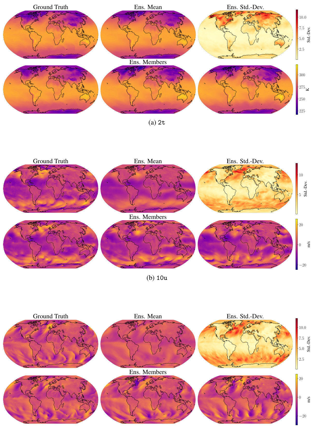
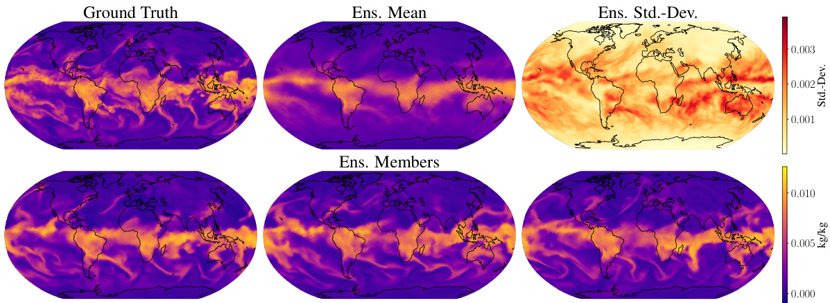
This figure shows an example of an ensemble forecast produced by the Graph-EFM model for specific humidity at 700 hPa (q700). The forecast is for a lead time of 10 days. The top row displays the ground truth, ensemble mean, and ensemble standard deviation. The bottom row shows three individual ensemble members randomly selected from the 80-member ensemble. This visualization helps to illustrate the model’s ability to capture forecast uncertainty by providing a range of possible future weather scenarios.

This figure compares the forecast results of four different models (GraphCast*, Graph-FM, Graph-EFM (ms), and Graph-EFM) against the ground truth for three different variables (u-component of 10 m wind, specific humidity at 700 hPa, and geopotential at 500 hPa) at a lead time of 10 days. For the probabilistic models (Graph-EFM and Graph-EFM (ms)), a single sample from the ensemble is shown, highlighting the variability within the model’s predictions.

This figure compares forecasts from GraphCast*, Graph-FM, Graph-EFM (ms) and Graph-EFM for three different variables at a 10-day lead time. The ground truth is also shown for comparison. For the probabilistic models, sampled ensemble members are displayed to illustrate the forecast uncertainty.

This figure compares the ground truth with forecasts from GraphCast*, Graph-FM, Graph-EFM(ms), and Graph-EFM models for three different variables at a 10-day lead time. It visualizes the forecasts for u-component of 10m wind, specific humidity at 700 hPa, and geopotential at 500 hPa. The probabilistic models (Graph-EFM and Graph-EFM(ms)) are represented by showing multiple sampled ensemble members, while the deterministic models (GraphCast* and Graph-FM) only display a single forecast.
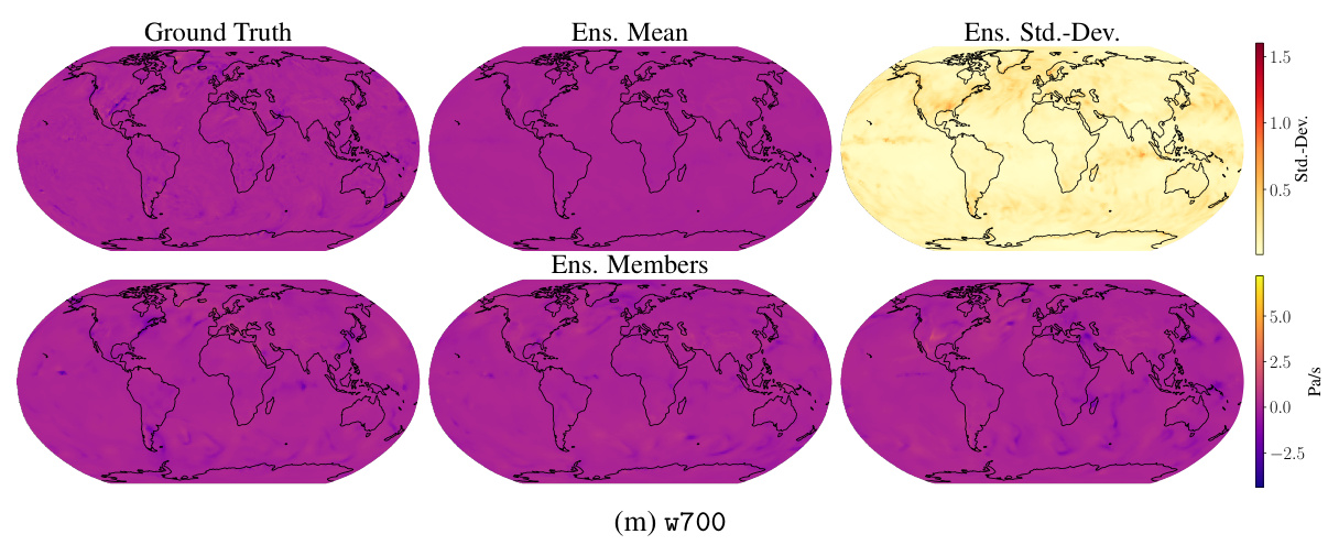
This figure displays example global ensemble forecasts generated by the Graph-EFM model at a lead time of 10 days. It shows the ground truth, the ensemble mean, the ensemble standard deviation, and three randomly selected ensemble members for several variables. The visualization allows for a comparison of the model’s predictions with the actual weather patterns.

This figure compares example forecasts from Graph-EFM and Graph-EFM (ms) models trained on MEPS data, focusing on lead time 57h. It showcases various weather variables (nlwrs, 2r, u65, v65) and illustrates the spatial coherence differences between the hierarchical Graph-EFM and the multi-scale Graph-EFM (ms). Graph-EFM demonstrates smoother, more realistic spatial patterns compared to Graph-EFM (ms), which exhibits patchier and less physically intuitive results.
This figure shows a schematic overview of the Graph-EFM model. It illustrates the flow of data through the hierarchical graph neural network. The figure specifically highlights the components for a limited area model, showing how the initial states and forcing inputs are processed through the different levels of the graph. The latent variables are sampled, and these affect the prediction made at each timestep. The global model overview is available in Appendix C, Figure 6.
This figure shows a schematic overview of the Graph-EFM model, illustrating the flow of data through the hierarchical graph neural network. It shows how the initial states and forcing data are processed through multiple GNN layers at different levels of the hierarchy to generate ensemble forecasts. The limited area model example is highlighted, showing the use of both boundary and grid data. A similar diagram for the global model is provided in Appendix C.

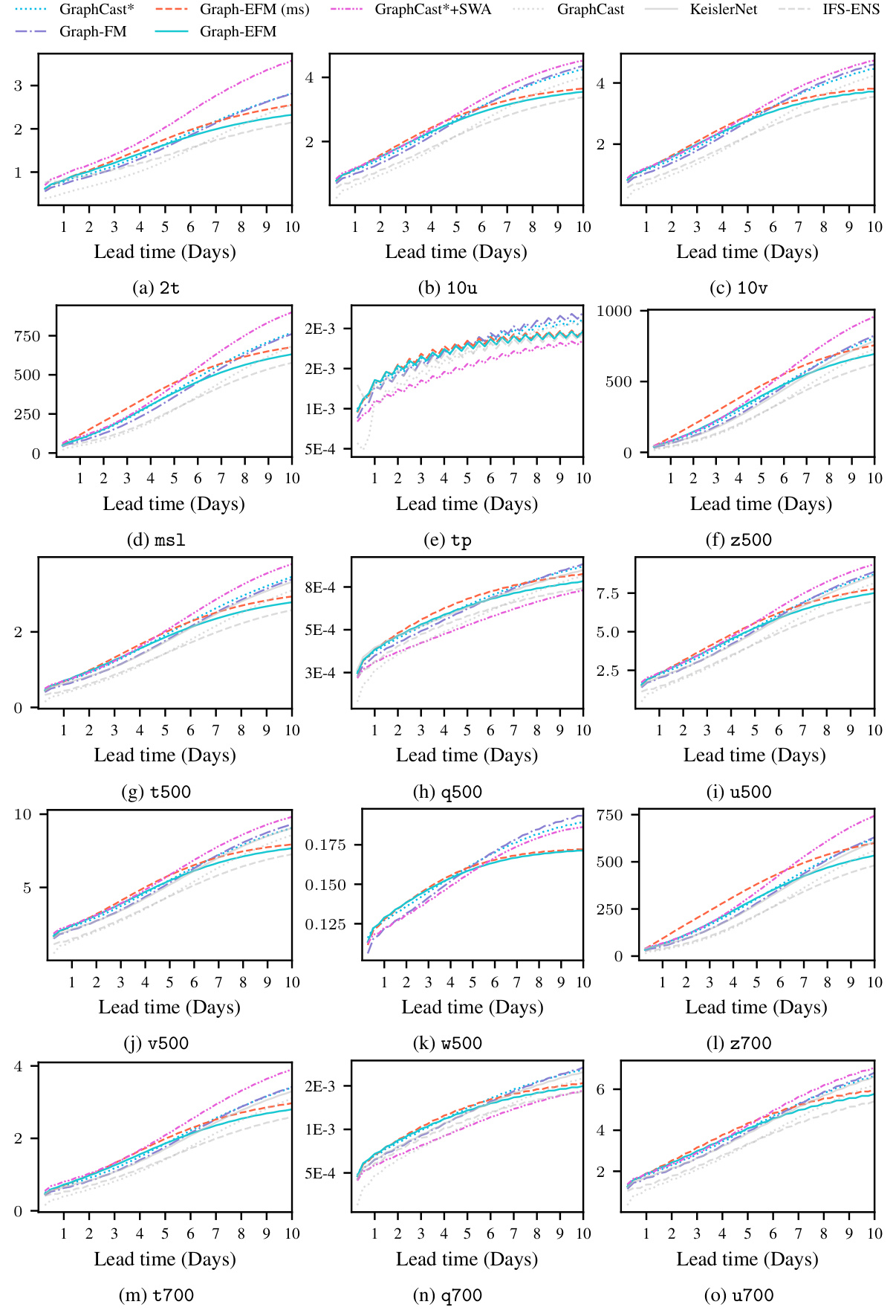
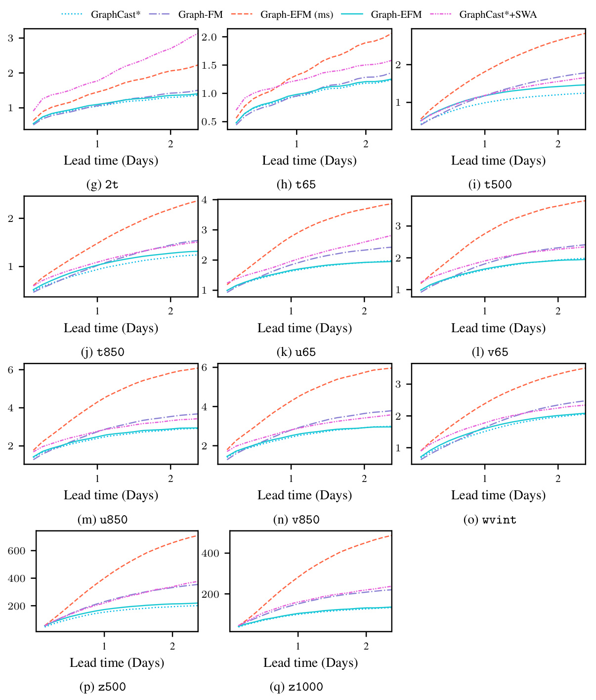
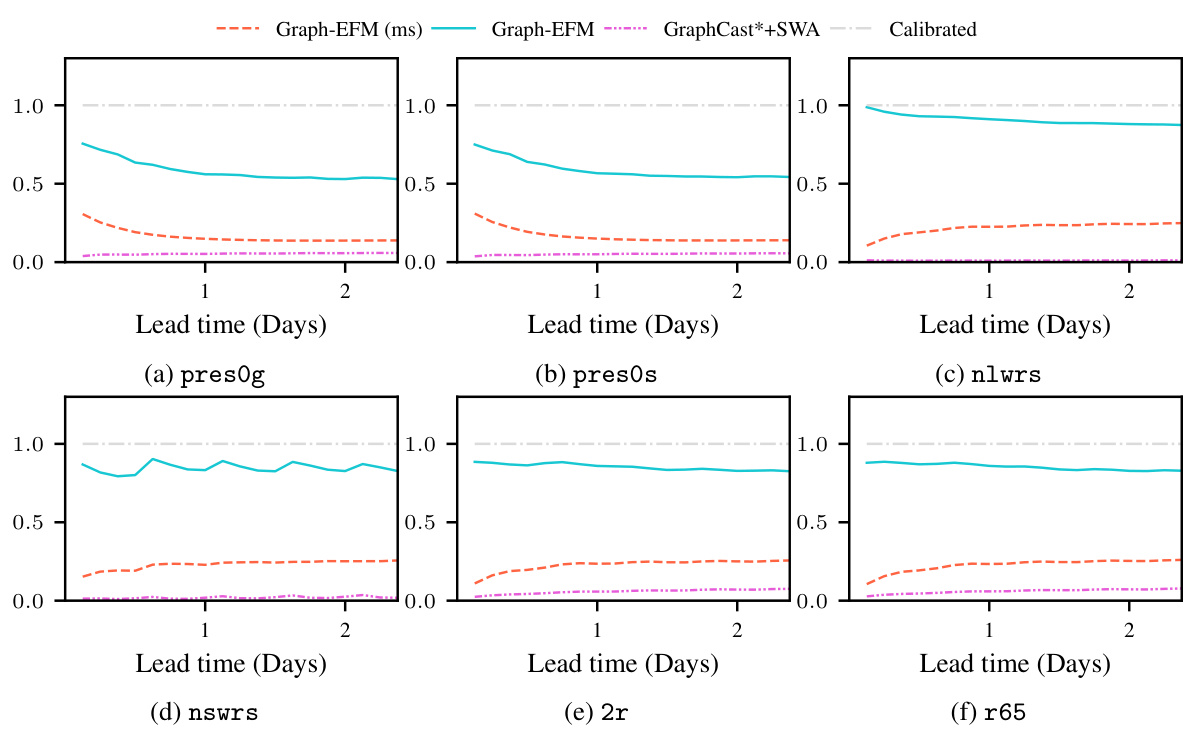
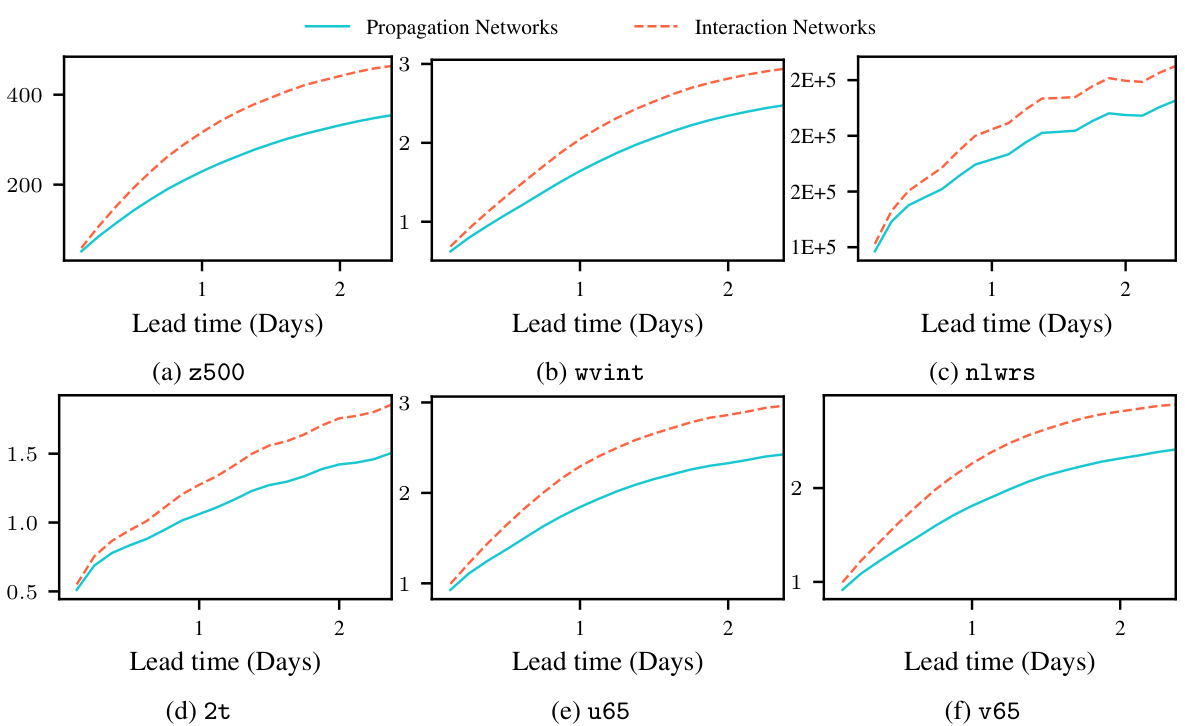
This figure compares the root mean square error (RMSE) results of Graph-FM models trained with Propagation and Interaction Networks on the ERA5 test dataset. The results are shown for different variables and lead times, providing a visual comparison of the performance of the two GNN approaches in the deterministic forecasting model.
This figure compares example forecasts from Graph-EFM and Graph-EFM (ms) for several variables at a lead time of 57 hours. It highlights the difference in spatial coherence between the models. Graph-EFM, using a hierarchical graph, produces smoother, more physically realistic forecasts compared to Graph-EFM (ms), which uses a multi-scale graph and shows patchier, less coherent results. The visual differences illustrate the impact of the graph structure on the model’s ability to capture spatial dependencies in weather forecasting.

This figure shows a schematic overview of the Graph-EFM model, illustrating how data flows through the model’s components in a Limited Area Model setting. It shows the hierarchical structure of the mesh graphs (G1, G2, G3), the latent variable (Zt), the predictor (Graph-FM), and the residual connections used to incorporate the previous state into the prediction. The figure also includes example data inputs and outputs, as well as an explanation of the sampling process used to generate an ensemble of forecasts. The caption also mentions that a similar figure for the global setting is available in Appendix C, Figure 6.
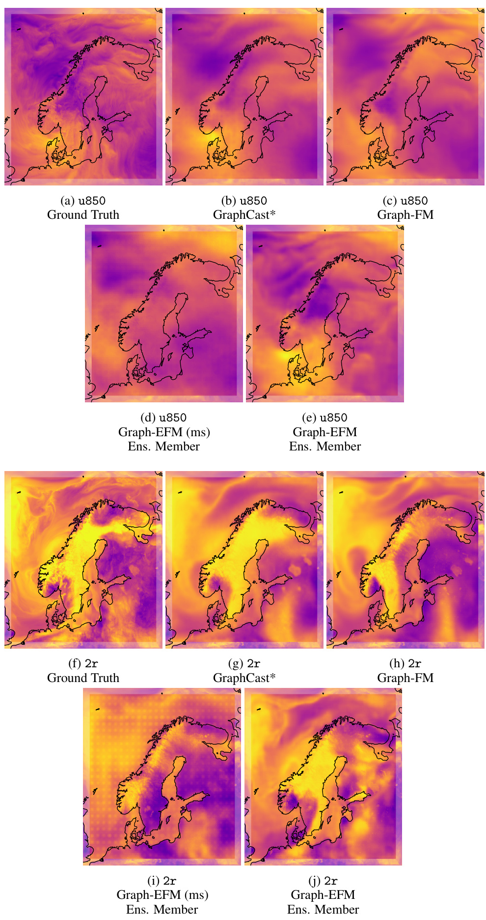
This figure compares the forecasts of u-component of wind at 850 hPa and 2 m relative humidity at 57h lead time from different models in the LAM experiment. The models compared include GraphCast*, Graph-FM, Graph-EFM (ms), and Graph-EFM. For the probabilistic models (Graph-EFM and Graph-EFM (ms)), sampled ensemble members are shown to illustrate the range of possible forecasts.

This figure shows example forecasts from Graph-EFM for the limited area model (LAM) at a lead time of 57 hours. It presents ground truth data alongside the ensemble mean, ensemble standard deviation, and multiple ensemble members for various weather variables. The purpose is to visually demonstrate the model’s ability to generate spatially coherent forecasts and capture uncertainty.
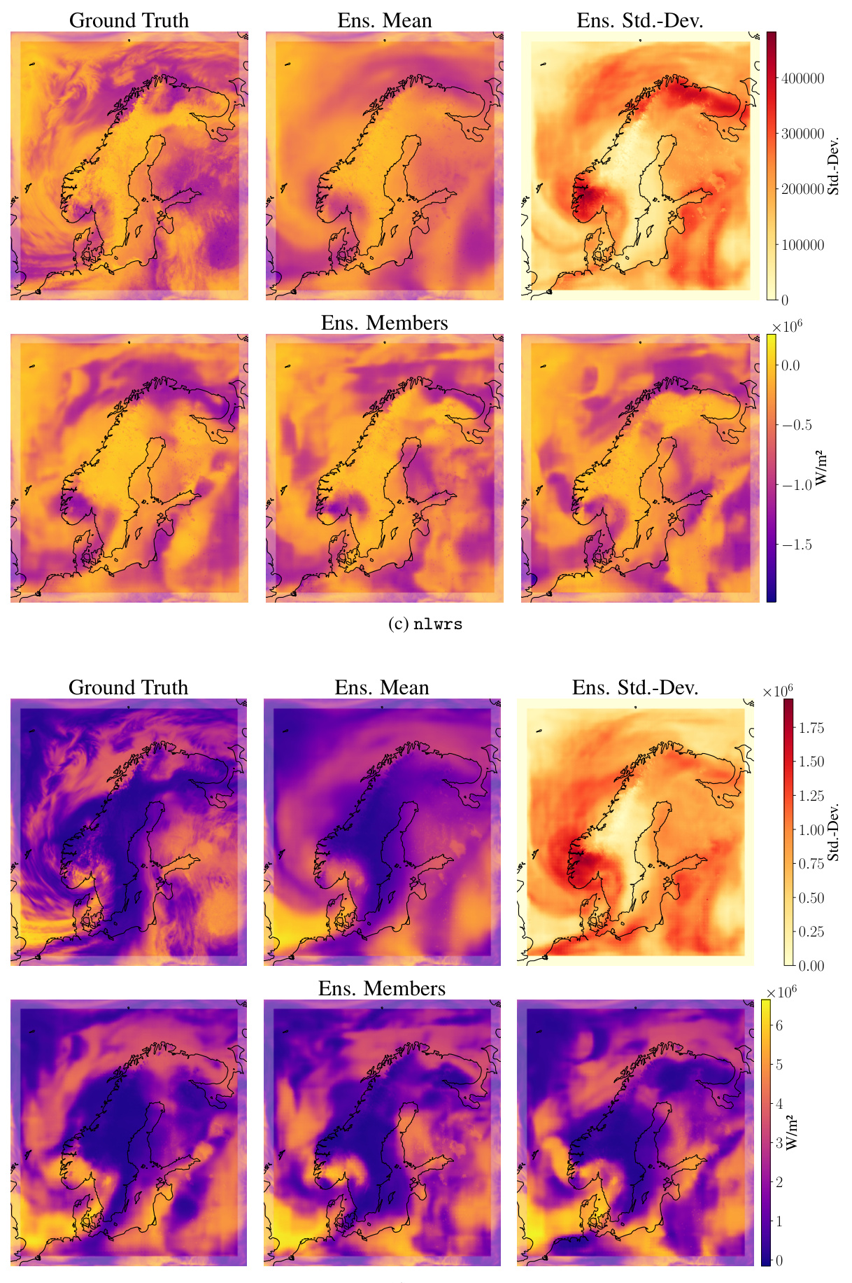
The figure shows example forecasts from Graph-EFM for the LAM setting at a lead time of 57h. It includes ground truth, ensemble mean, ensemble standard deviation, and three example ensemble members for the following variables: surface pressure (pres0g), surface pressure (pres0e), net longwave radiation (nlwrs), net shortwave radiation (nswrs), 2m relative humidity (2r), relative humidity at level 65 (r65), u-component of wind at 65 level (u65), v-component of wind at 65 level (v65), integrated column of water vapor (wvint), geopotential at 500 hPa (z500), geopotential at 1000 hPa (z1000), temperature at 65 level (t65), temperature at 500 hPa (t500), temperature at 850 hPa (t850), u-component of wind at 850 hPa (u850), v-component of wind at 850 hPa (v850), and vertical velocity at 700 hPa (w700). The forecasts highlight the model’s ability to capture both the mean state and the uncertainty in the forecasts.
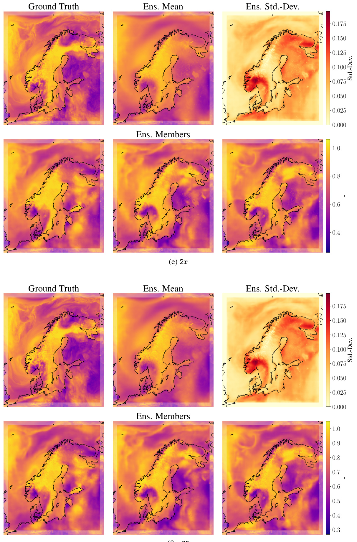
The figure shows example forecasts from the Graph-EFM model for the limited area modeling task. It shows the ground truth, ensemble mean, ensemble standard deviation, and three randomly chosen ensemble members for several variables, including pressure at ground level and sea level, net solar radiation flux (longwave and shortwave), relative humidity at 2 meters and 65 vertical levels, wind speed components (u and v) at 65 and 850 hPa, geopotential height at 500 and 1000 hPa, and integrated column of water vapor. These forecasts illustrate the model’s ability to capture both the mean and uncertainty in weather prediction at a high spatial resolution. The ensemble members demonstrate spatial coherence and realistic features of the forecasts.
The figure shows example forecasts from Graph-EFM for various weather variables at a lead time of 10 days. It includes the ground truth, ensemble mean, ensemble standard deviation, and three randomly selected ensemble members for each variable. The visualization helps to understand the model’s ability to capture forecast uncertainty and spatial coherence.
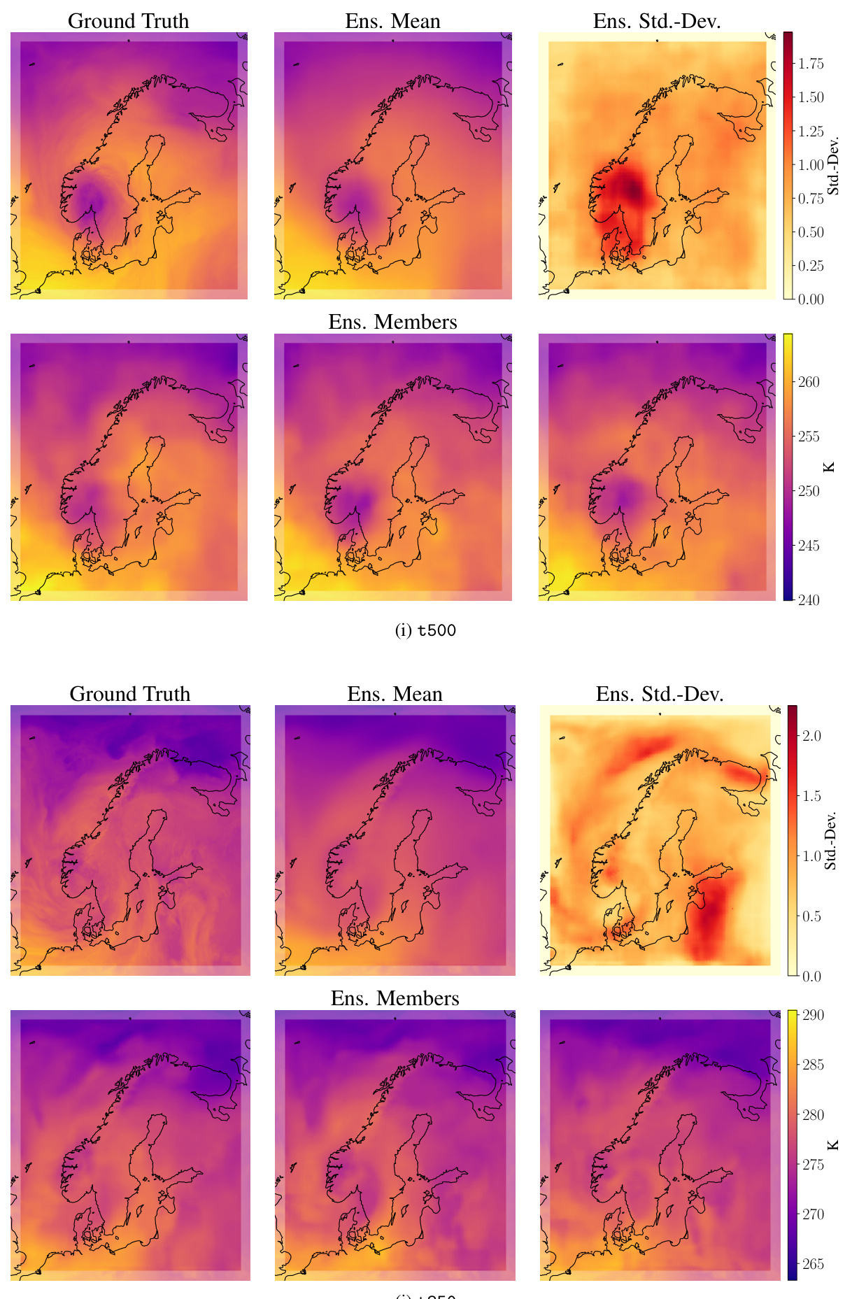
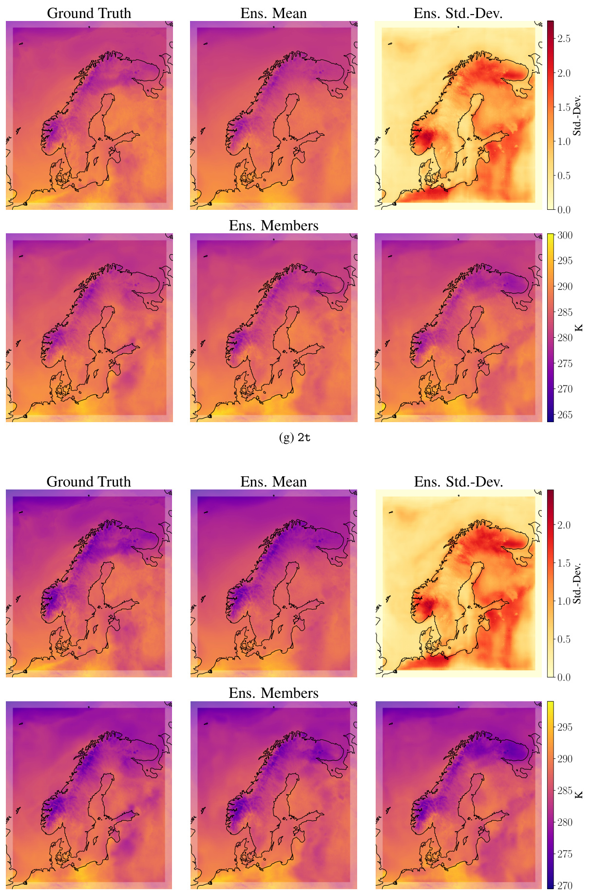
This figure displays example ensemble forecasts from the Graph-EFM model for the limited area modeling task using MEPS data. The forecasts are for a lead time of 57 hours. Each row shows a different variable: ground truth, ensemble mean, ensemble standard deviation, and three randomly selected ensemble members. The boundary area, which is not being forecast, is shown as a faded border around the plots. The figure visually demonstrates the spatial coherence of the ensemble forecasts produced by Graph-EFM, highlighting the model’s ability to capture the uncertainty and variability in weather prediction for a limited area.

This figure shows different mesh graphs used in the global forecasting experiments. Panel (a) through (d) show the mesh graphs G1 through G4, which are created by recursively splitting the faces of an icosahedron. Panel (e) shows the multi-scale mesh graph GMS, which combines all of these by connecting the nodes from G1 with edges from all the levels. Panel (f) shows the hierarchical mesh graph, which is structured differently than the multi-scale mesh graph; the nodes are not merged, but are structured hierarchically with edges connecting adjacent levels, as shown in panel (g). The earth’s surface is included for visualization but is not part of the model.

This figure shows the mesh graphs used in the global forecasting experiment of the paper. It includes four subfigures showing the different levels (G1, G2, G3, and G4) of the hierarchical mesh graph, along with a visualization of the multi-scale mesh graph (GMS) and a visualization of the hierarchical mesh graph. The caption notes that the vertical positioning of the nodes is for visualization purposes only and does not reflect their actual positions on the earth’s surface.

This figure shows example forecasts from Graph-EFM for the limited area modeling task using MEPS data. It displays ground truth values along with the ensemble mean, standard deviation, and several randomly selected ensemble members for various weather variables at a lead time of 57 hours. The purpose is to visually illustrate the model’s ability to generate spatially coherent and realistic ensemble forecasts for a limited geographical area.

This figure shows example forecasts from Graph-EFM for the LAM setting at a 57h lead time. It displays the ground truth, the ensemble mean, the ensemble standard deviation, and three randomly selected ensemble members for several meteorological variables. The purpose is to visually demonstrate the spatial coherence and variability captured by the Graph-EFM model in a limited area setting. Note that the forecasts include the boundary area, which is not included in the forecasting, presented as a faded border in each plot.

This figure shows different mesh graphs used in the global weather forecasting experiment described in the paper. It illustrates the multi-scale mesh graph (GMS) created by recursively splitting the faces of an icosahedron, as well as the hierarchical mesh graph used in the Graph-EFM model. The hierarchical graph is composed of multiple levels (G1, G2, G3, G4), with each level having a different spatial resolution, and it adds connections between the nodes of adjacent levels. The figure also shows an example of inter-level graph (G3,4), which demonstrates how information is propagated between the different levels in the hierarchical structure.
This figure provides a schematic overview of the Graph-EFM model, illustrating its components and data flow for a limited-area weather forecasting scenario. It shows how gridded weather data (Xt−2:t−1, Ft) and boundary forcing data (Bt) are fed into the model. The process involves mapping the data onto a hierarchical graph structure (G1, G2, G3), processing information through Graph Neural Networks (GNN) layers, and finally outputting a sample forecast (Xt) by sampling from the latent variable (Zt). A residual connection is used to incorporate the previous state. The figure highlights the key components of Graph-EFM, showcasing its hierarchical graph structure and efficient sampling method for generating ensemble forecasts. The global version of this model is discussed and illustrated in Figure 6 of Appendix C.

This figure shows a schematic overview of the Graph-EFM model, which is a probabilistic weather forecasting model. It uses a hierarchical graph neural network to efficiently sample spatially coherent forecasts. The figure shows the flow of data through the model, highlighting the different components, such as the latent variable model, the deterministic predictor, and the hierarchical graph structure. The left side shows an example for a limited area model, while the right side shows the same structure for a global model. The hierarchical structure is used to efficiently capture processes unfolding over different spatial scales. By sampling from a distribution over latent variables at the top of the hierarchy, the model is able to generate a large number of diverse forecasts.

This figure displays a case study of Hurricane Laura forecasting using Graph-EFM and deterministic models. It showcases 10m wind speed forecasts from ERA5 (ground truth), Graph-EFM (ensemble members and best-matching member), Graph-FM, and GraphCast*, at various lead times (7, 5, 3, and 1 days before landfall). The figure demonstrates the ability of the Graph-EFM ensemble to capture the hurricane’s development and landfall location, even with significant uncertainty at longer lead times, while deterministic models struggle to accurately predict the hurricane until much closer to landfall.

This figure shows the architecture of the Graph-EFM model for limited area forecasting. It illustrates the flow of data through the model’s hierarchical graph neural network structure, highlighting the use of latent variables and the process of sampling ensemble forecasts. The input consists of past weather states and forcing data, which are processed at multiple spatial scales by different graph layers. The model produces ensemble forecasts by sampling from the probability distribution of latent variables. A corresponding overview for the global setting is given in Figure 6 of Appendix C.
This figure shows an example of the Graph-EFM model’s forecast for specific humidity at 700 hPa (q700) with a lead time of 10 days. It visually compares the ground truth, ensemble mean, ensemble standard deviation, and three randomly selected ensemble members. The purpose is to illustrate the model’s ability to produce spatially coherent forecasts with uncertainty quantification.
This figure compares the forecasts of three different models (GraphCast*, Graph-FM, and Graph-EFM) with the ground truth for three different variables (10m wind, specific humidity at 700hPa, and geopotential at 500hPa) at a lead time of 10 days. For the probabilistic models (Graph-EFM and Graph-EFM(ms)), example members from the ensemble are shown to highlight the forecast uncertainty.
More on tables
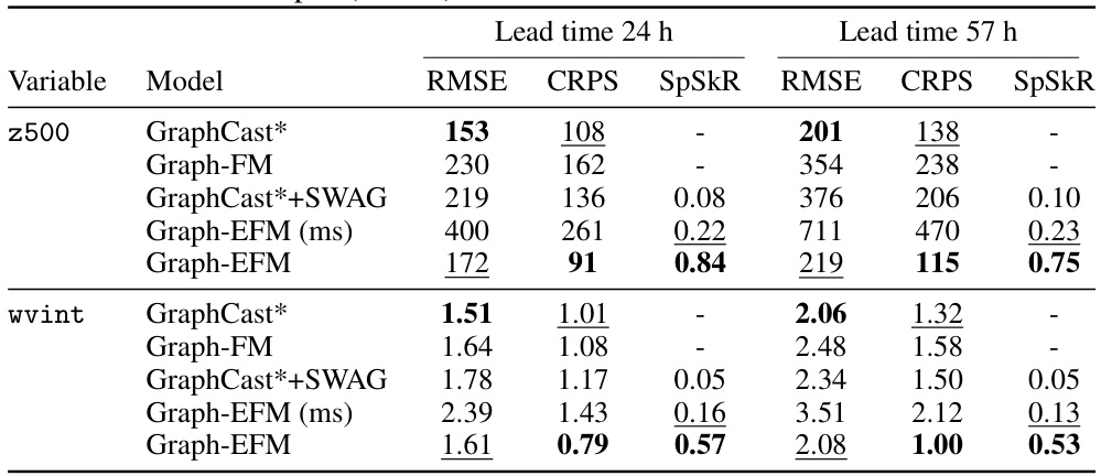
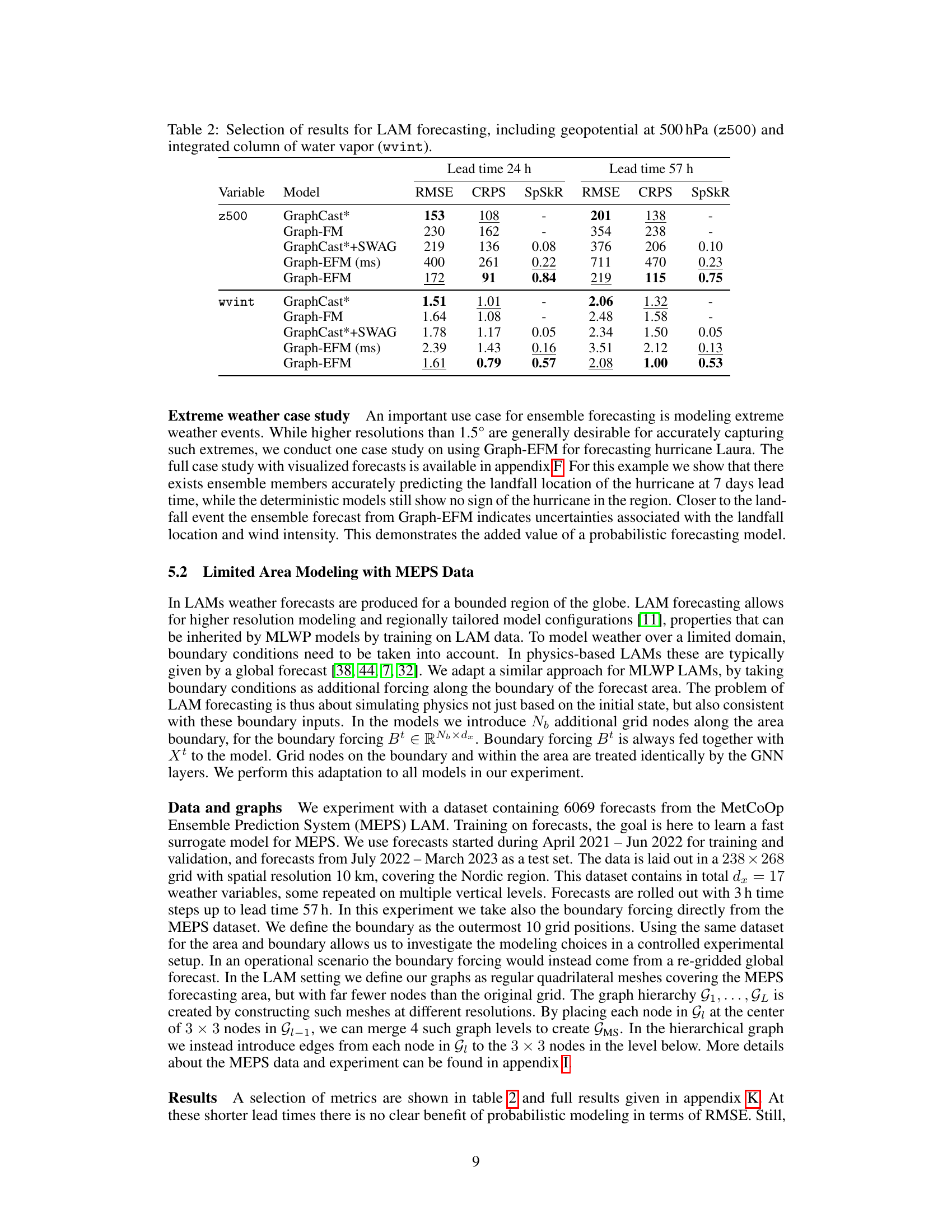
This table presents a subset of the results from the limited area modeling experiments. It shows the RMSE, CRPS, and SpSkR for two variables (geopotential at 500 hPa and integrated water vapor) at two different lead times (24h and 57h). The results are compared across several models, including the proposed Graph-EFM model and several baseline methods. Lower RMSE and CRPS values indicate better forecast accuracy, while a SpSkR value close to 1 indicates a well-calibrated ensemble.

This table presents a selection of the results from the global forecasting experiment. It compares several different models in terms of their Root Mean Squared Error (RMSE), Continuous Ranked Probability Score (CRPS), and Spread-Skill-Ratio (SpSkR) for two specific variables (geopotential at 500 hPa and 2-meter temperature) at lead times of 5 and 10 days. Lower RMSE and CRPS values indicate better model performance. A SpSkR close to 1 signifies a well-calibrated ensemble forecast, meaning the spread of the ensemble reflects the true uncertainty in the prediction.

This table presents a comparison of the performance of different weather forecasting models on global datasets. The models are evaluated based on several metrics: RMSE (Root Mean Squared Error), CRPS (Continuous Ranked Probability Score), and SpSkR (Spread-Skill-Ratio). Lower RMSE and CRPS values indicate better forecast accuracy. A SpSkR close to 1 suggests good calibration of the ensemble forecasts, meaning that the predicted uncertainty aligns well with the actual forecast error. The table shows results for two key variables: geopotential at 500 hPa (z500), a measure of atmospheric pressure, and 2m temperature (2t), which is temperature at 2 meters above the ground. Results are shown for different forecast lead times (5 days and 10 days).

This table presents the number of nodes and edges for each graph used in the global forecasting experiment. It breaks down the counts for the individual multi-scale graphs (G1-G5), the hierarchical graphs (G1-G4 and their inter-level connections), the final merged multi-scale graph (GMS), the bipartite graphs connecting the grid and mesh (GG2M and GM2G), and the total number of grid nodes.
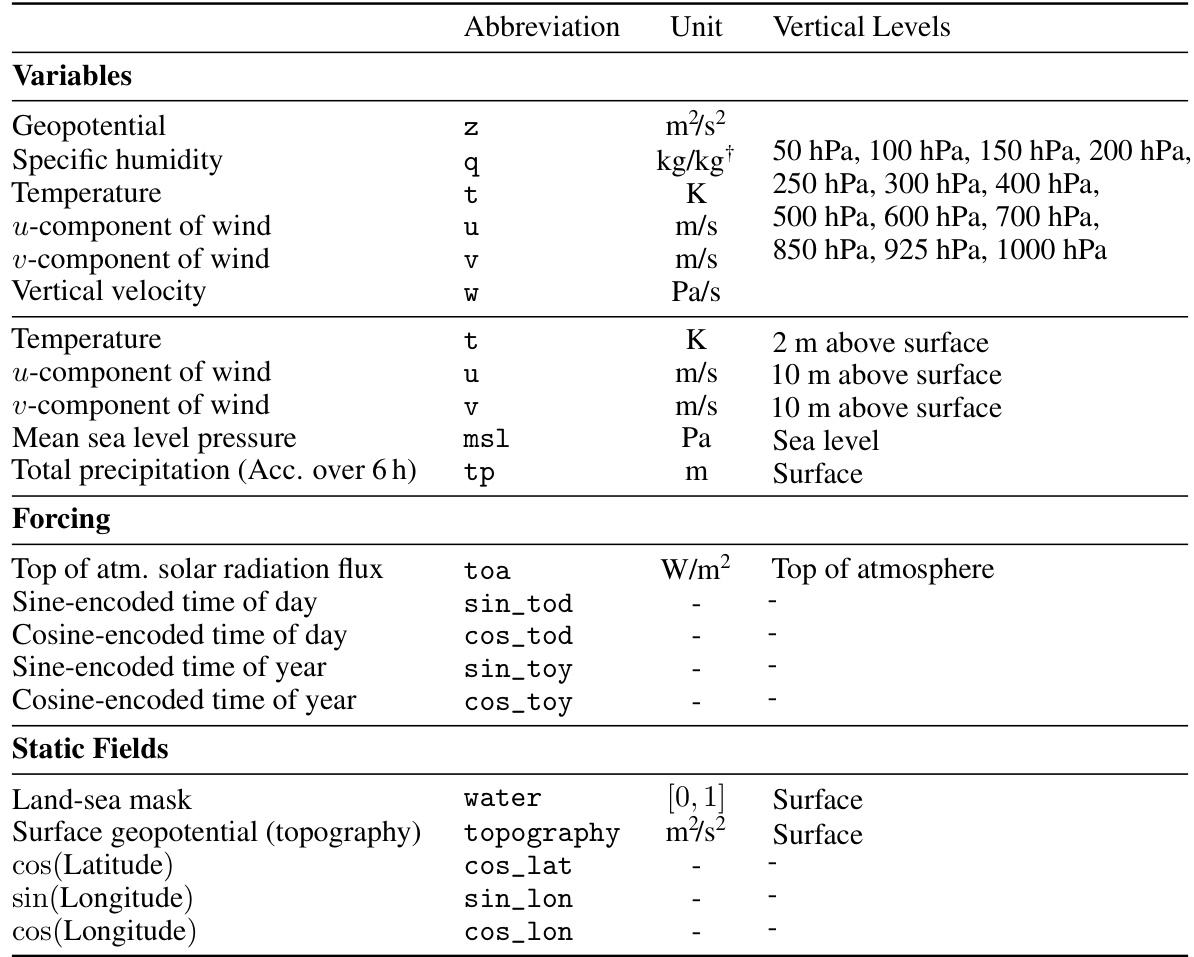
This table lists the variables, forcing, and static fields used in the global forecasting experiments of the paper. It shows the abbreviation, units, and vertical levels (where applicable) for each variable. The variables include geopotential, specific humidity, temperature, wind components, vertical velocity, and total precipitation. Forcing includes top of atmosphere solar radiation, sine and cosine encoded times of day and year. Static fields include the land-sea mask, surface topography, and latitude and longitude.

This table provides a summary of the model architectures used for global forecasting experiments in the paper. For each model, it lists the dimensionality of the representation vectors (dz), the number of processing steps performed on the mesh graph, the total number of parameters, and the total training time in GPU hours. The table includes the GraphCast*, Graph-FM, Graph-EFM (ms), and Graph-EFM models.
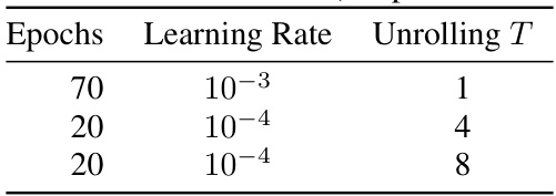
This table shows the training schedule used for the deterministic models, GraphCast* and Graph-FM, when trained on global data. It details the number of epochs, learning rate, and the unrolling length (T) used during different phases of the training process. The learning rate is decreased in steps as the training progresses, with a longer unrolling length being used in later stages of training.
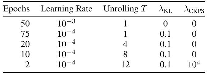
This table shows the training schedule used for the Graph-EFM model in the global forecasting experiments. It details the number of epochs, learning rate, unrolling time steps (T), and weighting hyperparameters (λKL and λCRPS) used for different stages of the training process. A similar schedule was used for Graph-EFM(ms) but with different values for λKL and λCRPS.
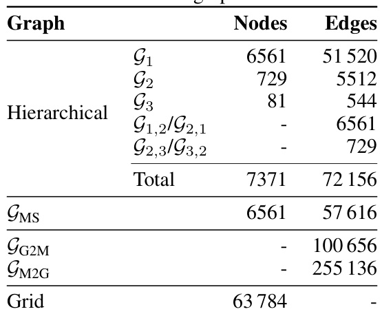
This table presents the number of nodes and edges in each of the graphs used in the MEPS experiment. It shows the statistics for the hierarchical graph (G1, G2, G3, G1,2/G2,1, G2,3/G3,2), the multi-scale graph (GMS), the bipartite graphs connecting the grid and the mesh (GG2M, GM2G), and the grid itself. These graphs are used in the Graph-based Ensemble Forecasting Model (Graph-EFM) for the limited area modeling task.

This table lists the variables, forcing, and static fields used in the MEPS dataset for the limited area modeling experiments. It specifies the units and vertical levels for each variable and also provides information about the ground level, sea level, and surface variables. The table is important for understanding the data used in the experiments described in the paper.

This table presents the details of the model architectures used for limited area modeling (LAM) forecasting, along with their training times. It includes information about the dimensionality of the representation vectors (dz), the number of processing steps in the GNN layers, the total number of parameters in each model, and the training time in GPU hours. The table provides a comparison of the computational requirements of different models used in the LAM forecasting experiments.

This table shows the training schedule used for the deterministic models, GraphCast* and Graph-FM, when trained on global data. It specifies the number of epochs, the learning rate, and the unrolling T used during the training process.

This table shows the training schedule used for the Graph-EFM model on the MEPS dataset. It details the number of epochs, learning rate, unrolling time steps (T), and weighting hyperparameters (λKL and λCRPS) for each stage of the training process. A similar schedule was used for the Graph-EFM(ms) model, but with different values for the hyperparameters.
Full paper#
