↗ OpenReview ↗ NeurIPS Proc. ↗ Chat
TL;DR#
Understanding complex relationships between brain activity and behavior is a major challenge in neuroscience. While latent variable models are effective for dimensionality reduction, generating realistic neural spiking data, especially behavior-dependent data, remains difficult. This is due to the high dimensionality and discrete nature of spiking data, combined with the need for behavior-dependent generation.
The paper introduces Latent Diffusion for Neural Spiking data (LDNS), a novel generative model that solves this problem. LDNS uses an autoencoder with structured state-space layers to project high-dimensional spiking data into a continuous latent space. Then, expressive diffusion models generate neural activity with realistic statistics. LDNS is validated on synthetic and real data, including variable-length recordings from humans and monkeys, demonstrating its ability to generate realistic spiking data given reach direction or unseen reach trajectories. This model significantly improves our ability to simulate neural activity and test hypotheses.
Key Takeaways#
Why does it matter?#
This paper is crucial for neuroscience researchers due to its novel Latent Diffusion for Neural Spiking data (LDNS) model. LDNS allows for high-fidelity generation of neural activity while simultaneously providing access to low-dimensional latent representations. This opens exciting new possibilities for simulating experimentally testable hypotheses and developing more realistic brain models.
Visual Insights#
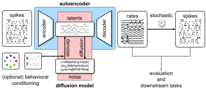
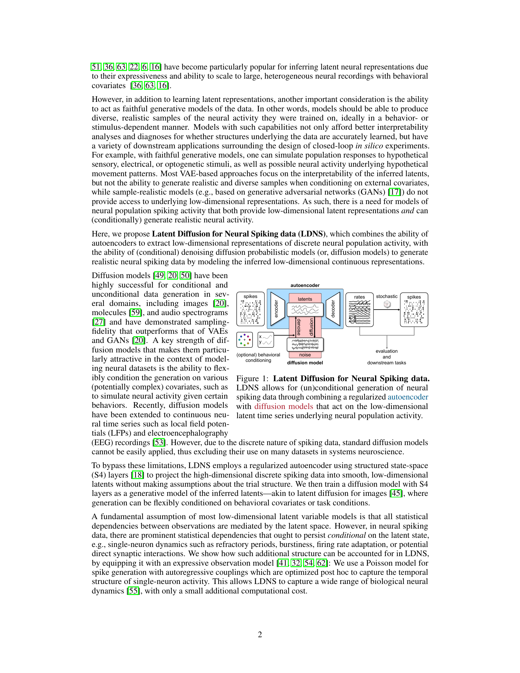
This figure illustrates the architecture of Latent Diffusion for Neural Spiking data (LDNS). LDNS uses a two-stage process. First, a regularized autoencoder processes neural spiking data to generate low-dimensional continuous latent representations. These latents capture the essential structure of the neural activity. Second, a diffusion model operates on these latent representations to generate new, realistic samples of neural activity. The process is flexible and allows for both unconditional and conditional generation, based on external behavioral covariates (represented by y). The figure includes blocks for the encoder, decoder, diffusion model, and noise. The output is then stochastically converted into spike trains, which can be further evaluated.

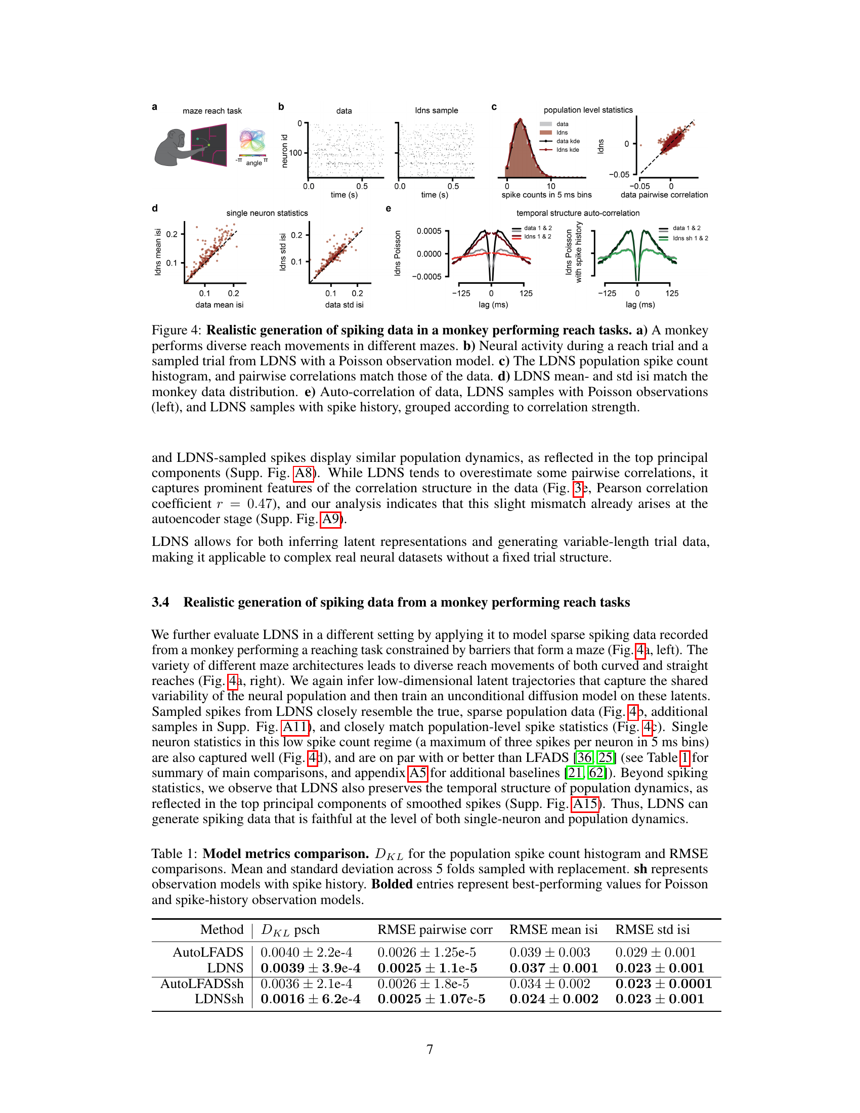
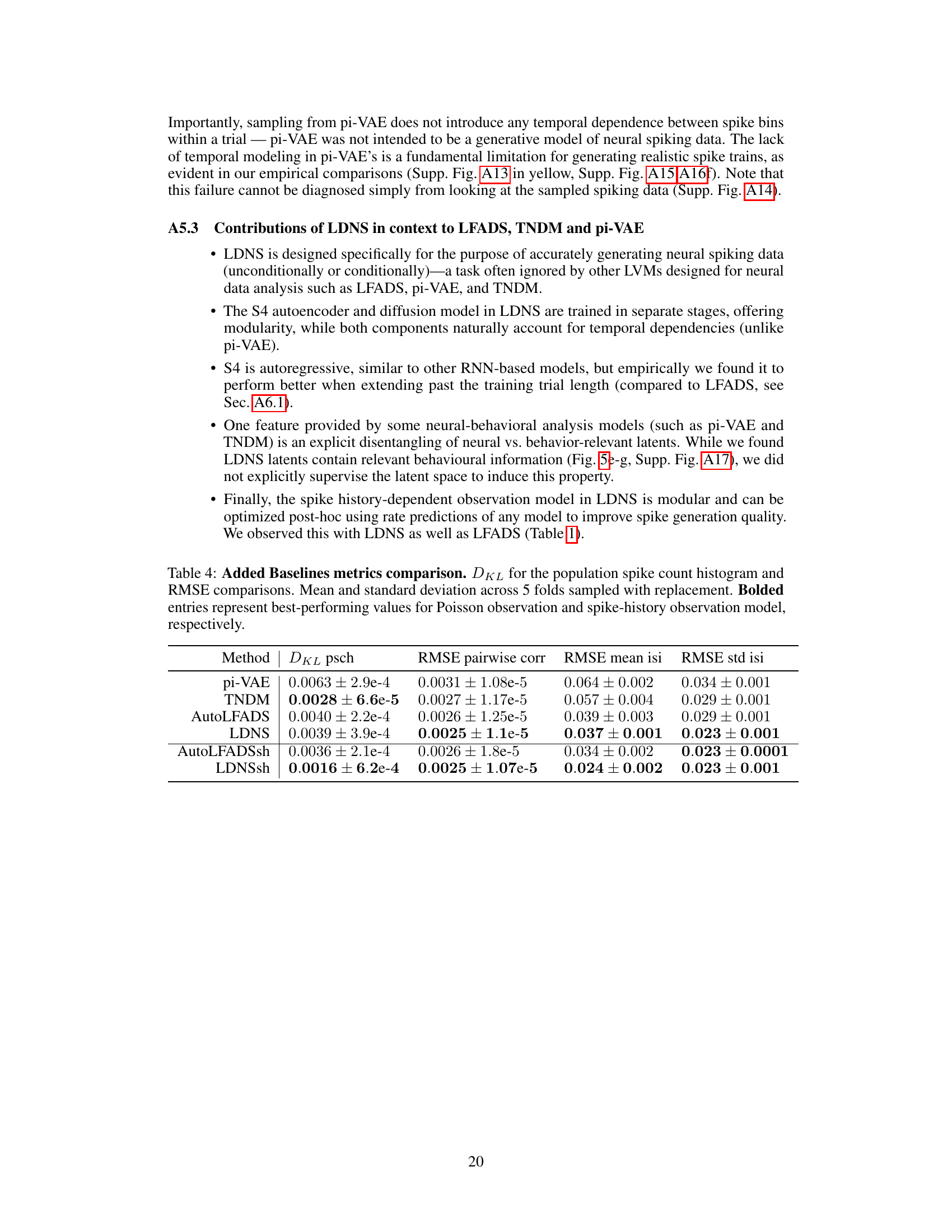
This table presents a comparison of different model’s performance based on several metrics: DKL (Kullback-Leibler divergence) for the population spike count histogram, and RMSE (Root Mean Squared Error) for pairwise correlations, mean inter-spike intervals (isi), and standard deviation of isi. The comparison includes four models: AutoLFADS (a baseline), LDNS (the proposed method), AutoLFADSsh (AutoLFADS with a spike history-dependent observation model), and LDNSsh (LDNS with a spike history-dependent observation model). The results are averaged over five folds, each with replacement sampling. The bold values indicate the best performance for the Poisson and spike-history observation models respectively.
In-depth insights#
Spiking Data Gen#
Spiking Data Gen, if interpreted as generative models for neural spiking data, represents a significant area of research. The challenge lies in creating models that accurately capture the complex, stochastic nature of neural activity, including realistic spike patterns and temporal correlations. Successful approaches would likely leverage advances in deep learning, potentially incorporating techniques like diffusion models or VAEs. Key considerations include handling the high dimensionality of spiking data, managing variable-length recordings, and incorporating relevant behavioral context. Ideally, a successful Spiking Data Gen model should enable controlled generation of neural activity under specific conditions, offering valuable tools for hypothesis testing and in-silico experimentation. Achieving high fidelity in the generated data is critical for downstream applications, such as testing decoding algorithms or investigating network dynamics under diverse scenarios. However, the complexities of neural spiking make this a challenging task, requiring careful consideration of statistical properties, computational efficiency, and the interpretability of generated data.
LDNS Model#
The LDNS model presents a novel approach to generative modeling of neural spiking data by combining the strengths of autoencoders and diffusion models. Autoencoders are used to map high-dimensional, discrete spiking data into a lower-dimensional, continuous latent space, facilitating efficient representation and manipulation of the data. Diffusion models operating in this latent space generate new, realistic spiking patterns. The use of structured state-space (S4) layers within both the autoencoder and diffusion model is crucial for effectively handling the temporal dependencies inherent in neural spiking data, allowing for the generation of variable-length sequences. Furthermore, an expressive observation model is incorporated to address dependencies within the data not captured by the latent representation, enhancing the realism of the generated spiking patterns. The LDNS model’s ability to generate realistic neural activity under both unconditional and conditional settings (e.g., given behavioral covariates) showcases its flexibility and potential in simulating experimental hypotheses and exploring neural dynamics. Conditional generation is a significant advantage, enabling the simulation of responses to various stimuli or behaviors, making the model a valuable tool in neuroscience research.
Autoencoder Role#
The autoencoder plays a crucial role in the LDNS framework by acting as a bridge between high-dimensional, discrete neural spiking data and a lower-dimensional, continuous latent space. Its primary function is dimensionality reduction, transforming complex neural activity into a more manageable representation suitable for processing by the diffusion model. This compression is essential for efficient generation, especially with long time series and complex behavioral covariates. Regularization techniques incorporated into the autoencoder design ensure that the latent representations are smooth and meaningful, preventing overfitting and promoting generalization to unseen data. The autoencoder’s structured state-space (S4) layers are especially important, allowing it to capture temporal dynamics in the neural data, leading to more realistic and temporally coherent generated spiking patterns. Furthermore, the autoencoder’s output, representing firing rates, serves as a foundation for building a Poisson observation model, improving the realism of the generated spike trains. By effectively projecting the data into a low-dimensional latent space, the autoencoder is pivotal in enabling the generation of realistic and interpretable neural spiking activity by the diffusion model.
Variable Trials#
The concept of ‘Variable Trials’ in a research paper likely refers to experimental designs where the duration or number of observations within each trial isn’t fixed. This contrasts with traditional fixed-trial designs, which maintain consistent trial lengths. Variable trials offer increased ecological validity, mirroring real-world scenarios more accurately. However, they also present analytical challenges. Standard statistical methods often assume a constant trial length, leading to biases and inaccuracies if applied directly to variable-length data. Addressing this requires advanced statistical techniques, such as time-series analysis or methods that can handle missing data. Careful consideration must be given to how to properly align and compare data across trials of differing lengths. The paper likely explores innovative approaches to analyzing variable trial data, possibly employing methods like dynamic time warping or latent variable models to extract meaningful information despite the variability in trial lengths. Successfully handling variable trial data enhances the generalizability and practical significance of the research findings, moving beyond simplified laboratory settings towards more naturalistic observations. The implications for computational resources, model complexity, and the need for robust algorithms must also be considered.
Future Scope#
The future scope of latent diffusion models for neural spiking data involves several promising directions. Improving model scalability to handle recordings with an even greater number of neurons and longer durations is crucial. This requires efficient algorithms and potentially new architectural designs. Exploring different neural network architectures beyond the S4 layers used in LDNS could enhance model performance and flexibility. The development of more sophisticated observation models to accurately capture complex single-neuron dynamics is also vital, potentially using more advanced point processes. Incorporating diverse types of neural data beyond spiking activity, such as LFPs or calcium imaging data, within a unified generative framework would greatly expand the model’s capabilities. A significant advancement would be to develop methods for efficient conditional generation that seamlessly integrates with experimental design and hypothesis testing. Finally, rigorous benchmarking and evaluation against a wider range of baselines and datasets are essential to fully assess the capabilities and limitations of latent diffusion models for this specific application.
More visual insights#
More on figures
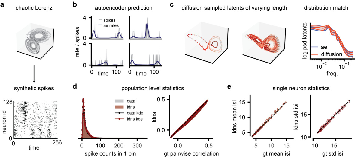
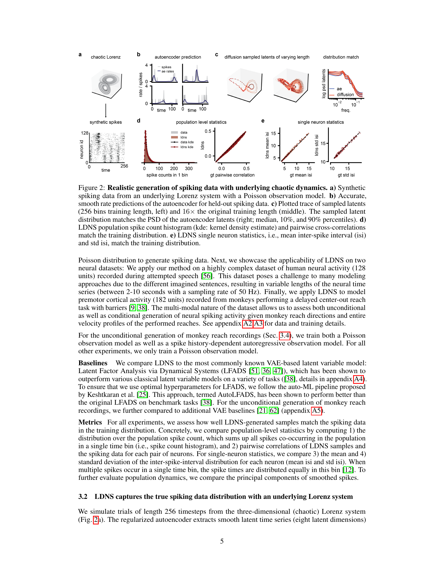
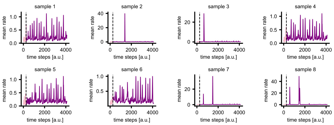
This figure demonstrates the performance of LDNS on synthetic data generated from a chaotic Lorenz system. It shows that LDNS accurately recovers latent structure, firing rates, and spiking statistics at both the population and single-neuron levels, even when generating data of significantly longer duration than seen during training.

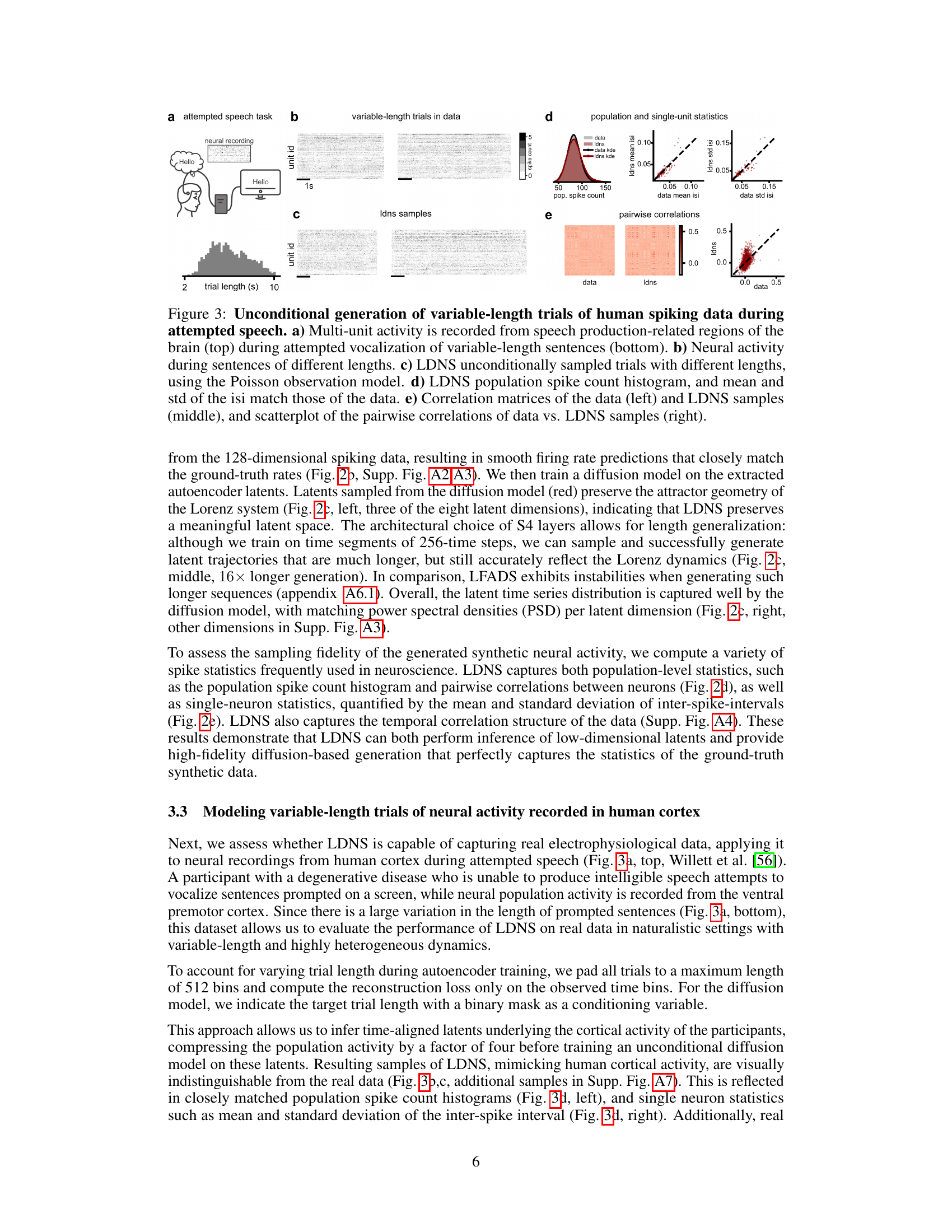
This figure demonstrates the unconditional generation of variable-length neural spiking data using LDNS. Panel (a) shows the experimental setup where neural activity was recorded during attempted speech, highlighting the variable length of sentences. Panel (b) displays example neural recordings of varying lengths. Panel (c) presents the variable-length samples generated by LDNS, using the Poisson observation model. Panels (d) and (e) provide quantitative comparisons between the generated data and the real data, focusing on population-level statistics (spike counts, inter-spike intervals), and pairwise correlations between neurons. The results indicate that LDNS successfully captures the statistical properties of the original dataset, demonstrating its ability to generate realistic and variable-length neural activity.
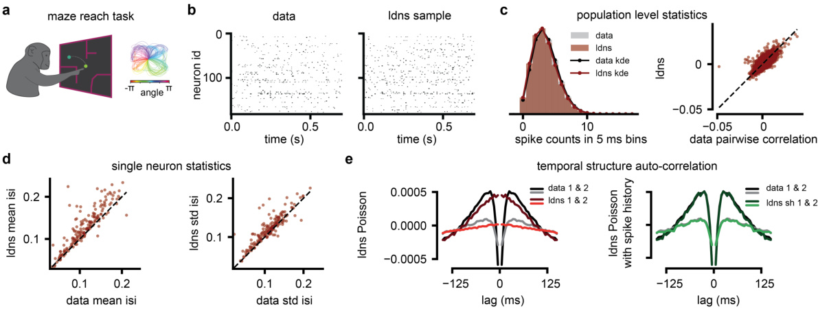
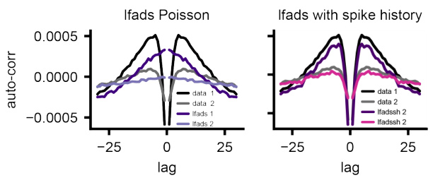
This figure demonstrates the ability of the LDNS model to generate realistic spiking data for a monkey performing reach tasks in different mazes. Panel (a) shows a schematic of the experimental setup. Panel (b) compares real neural activity with data generated by LDNS, demonstrating high similarity. Panel (c) shows that LDNS accurately captures population-level statistics such as spike count distributions and pairwise correlations. Panel (d) shows that LDNS also reproduces single-neuron statistics such as the mean and standard deviation of inter-spike intervals. Finally, panel (e) compares the temporal autocorrelation structure of real and generated data, highlighting that incorporating spike history into the model improves the accuracy of the generated data.
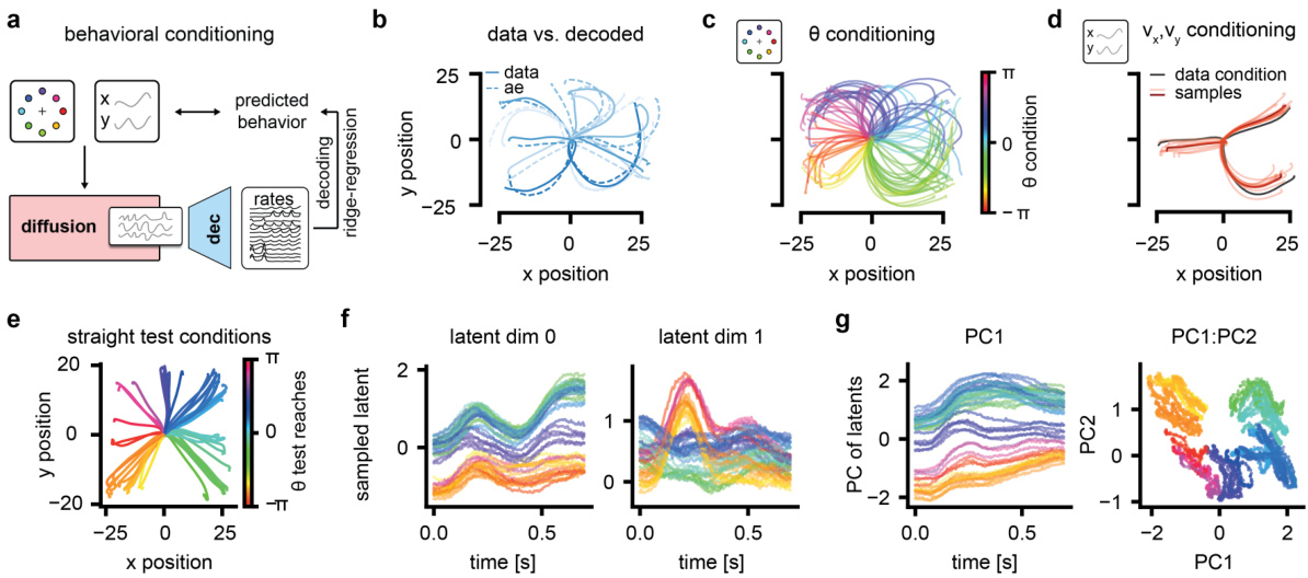
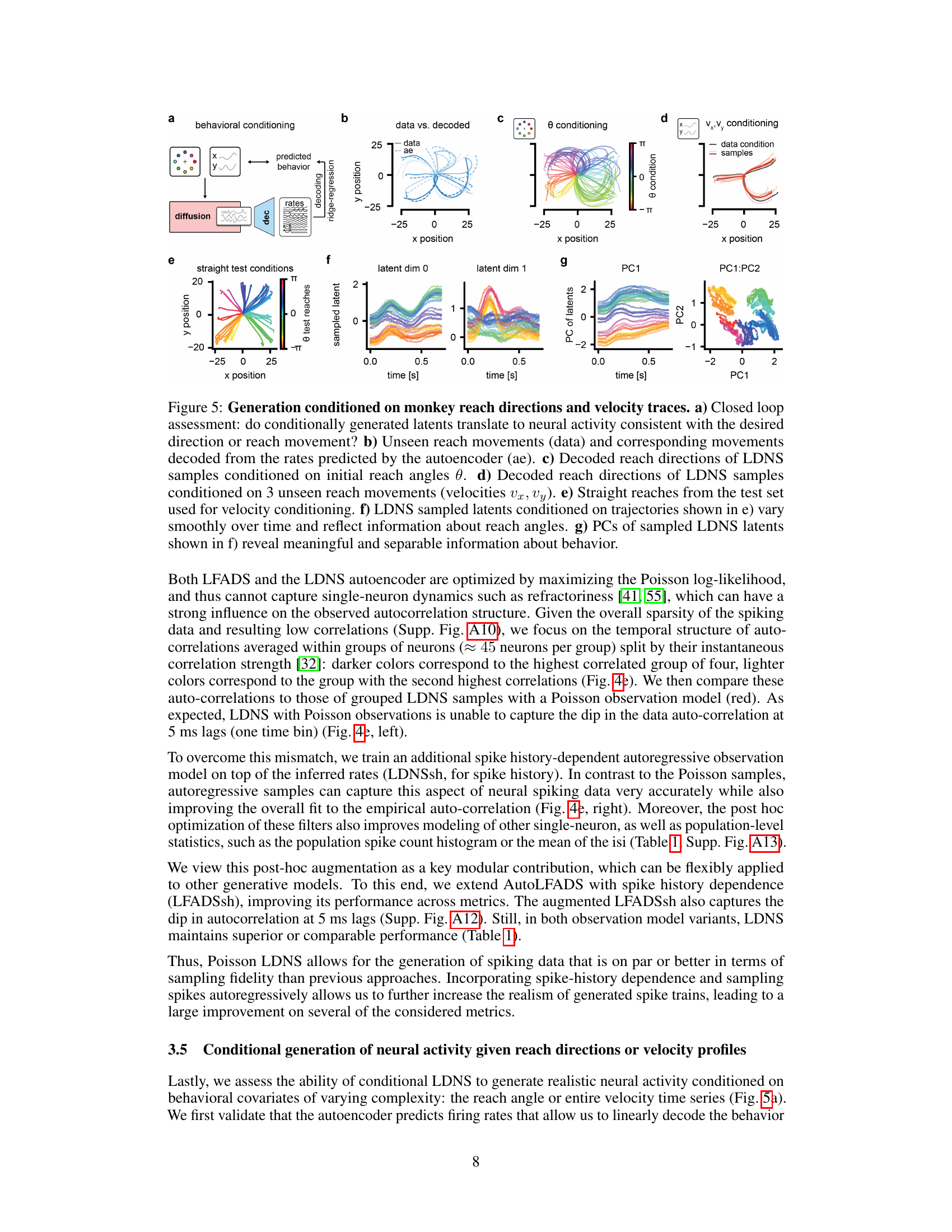
This figure demonstrates the conditional generation capabilities of LDNS. Panel (a) outlines the closed-loop experimental design. Panels (b-d) show that LDNS can generate realistic neural activity when conditioned on either reach direction (b,c) or full reach trajectories (d). Panels (e-g) show how LDNS captures the underlying behavioral information within its latent representation; latent trajectories vary smoothly over time and reflect reach direction and velocity.
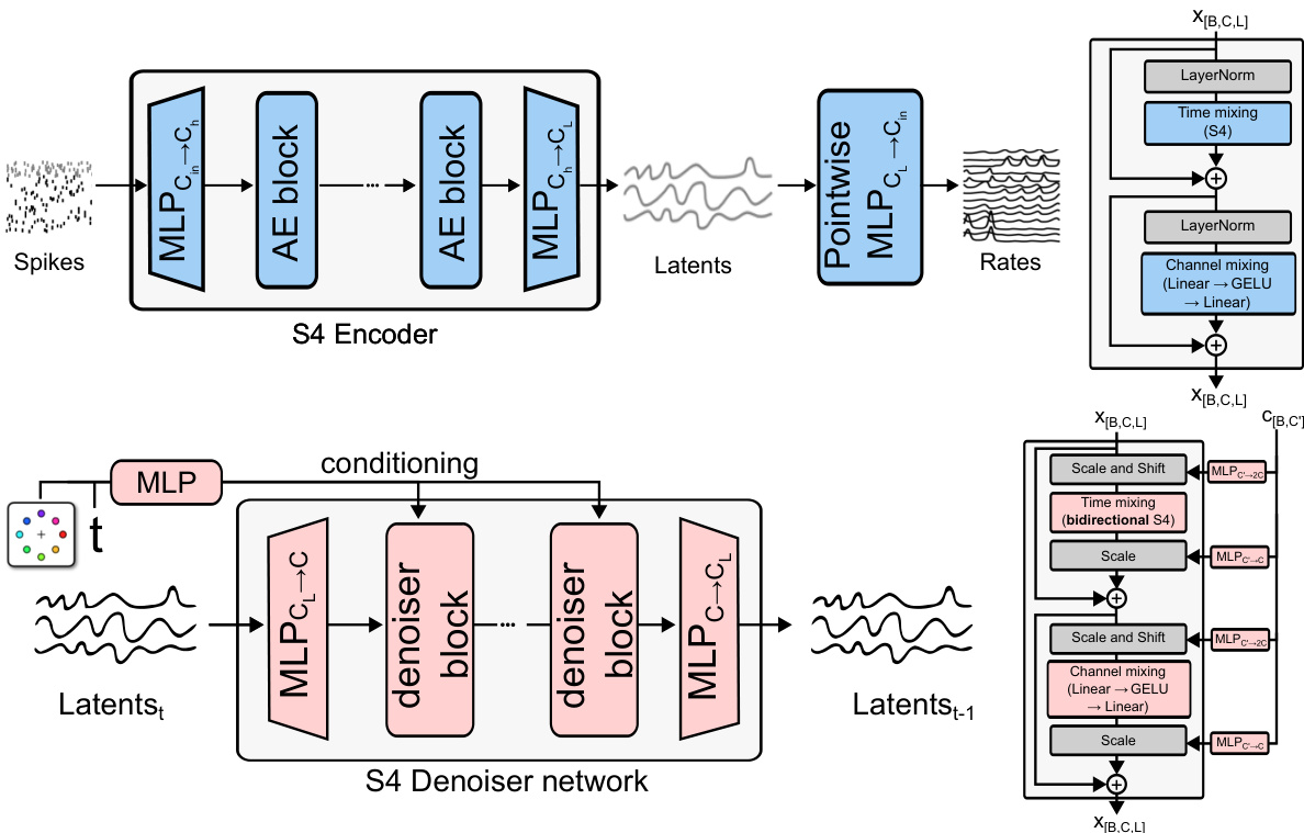
The figure illustrates the architecture of Latent Diffusion for Neural Spiking data (LDNS). LDNS is a two-stage model. The first stage uses a regularized autoencoder with structured state-space (S4) layers to encode high-dimensional, discrete neural spiking data into a low-dimensional, continuous latent space representation. The second stage utilizes a diffusion model, trained on these latent representations, to generate new neural spiking data. This generation process can be conditioned on behavioral covariates to produce behaviorally relevant neural activity. The figure shows the flow of data through the encoder, latent space, diffusion model, and decoder, highlighting the key components and their interactions.
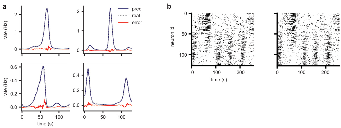
This figure demonstrates the performance of LDNS on a synthetic dataset generated from a chaotic Lorenz system. It showcases the model’s ability to accurately generate spiking data that matches the statistical properties of the original data at both population and single-neuron levels. The autoencoder accurately predicts firing rates, and the diffusion model generates samples with realistic firing statistics and latent dynamics.
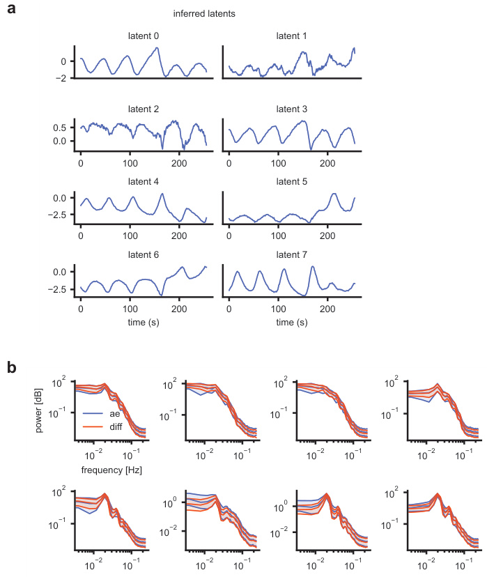
This figure demonstrates the ability of the S4 autoencoder to extract smooth, low-dimensional latent representations from high-dimensional discrete neural spiking data. Panel (a) shows inferred latents for a single test sample, highlighting the smoothness achieved by the autoencoder. Panel (b) compares the power spectral density (PSD) of the autoencoder’s inferred latents (during training) with the PSD of latents sampled from the trained diffusion model. The close match indicates that the diffusion model successfully captures the distribution of the inferred latent space.
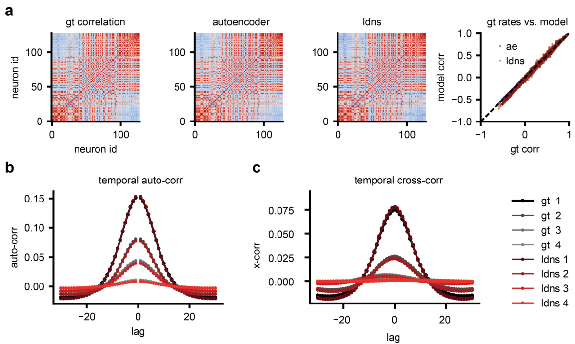
This figure demonstrates that LDNS accurately recovers the correlation structure of the synthetic data generated from the Lorenz system. Panel (a) shows that both the autoencoder and LDNS-generated samples accurately reflect the instantaneous correlations between neurons. Panel (b) compares the autocorrelations (correlations of a neuron with itself over time) of the ground truth data and LDNS samples, demonstrating a near-perfect match. Similarly, panel (c) shows that the cross-correlations (correlations between different neurons) are also accurately reproduced by LDNS.
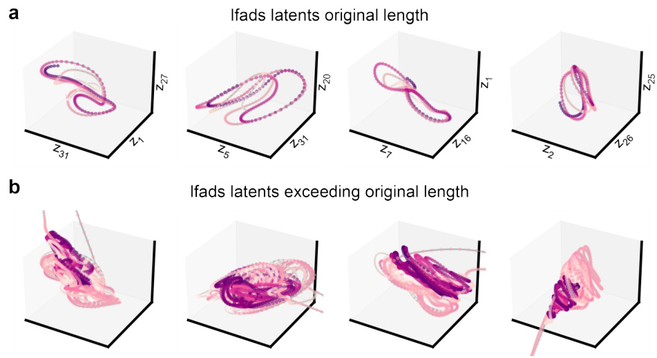
This figure demonstrates the ability of Latent Diffusion for Neural Spiking data (LDNS) to generate realistic spiking data from an underlying chaotic Lorenz system. It shows that LDNS accurately recovers the latent structure, firing rates, and spiking statistics of the synthetic data, even when generating variable-length data. The autoencoder accurately predicts firing rates, and the diffusion model samples latents that match the power spectral density of the autoencoder latents. Population-level and single-neuron spiking statistics from LDNS also closely match the training data. This showcases the model’s ability to generate realistic spiking data with complex dynamics.
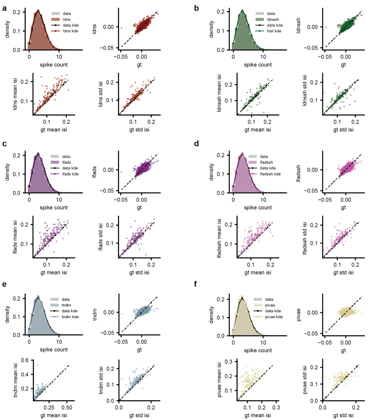
The figure compares population-level and single-neuron-level statistics of different models: LDNS (with and without spike history), LFADS (with and without spike history), TNDM, and pi-VAE. For each model, it shows kernel density estimations of population spike counts, mean inter-spike intervals (ISIs), and standard deviations of ISIs, along with scatter plots comparing the model’s predictions to the ground truth data. This visualizes how well each model captures the distribution and characteristics of the neural spiking data.
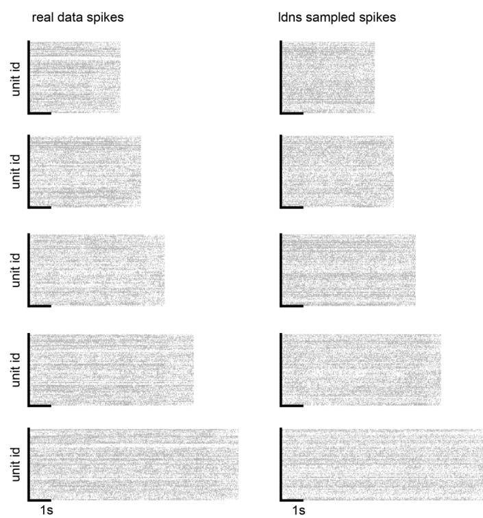
This figure compares five example trials of real neural spiking data with five corresponding samples generated by the LDNS model. The figure visually demonstrates the model’s ability to generate realistic-looking spiking activity that resembles the characteristics of the real data. Each row shows a single trial, both the original and the LDNS-generated version, allowing for a direct visual comparison of the spike patterns.
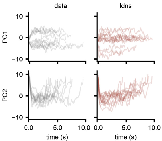
This figure compares the latent space trajectories obtained from LDNS model with those obtained from the autoencoder. It shows both unconditionally inferred latents and those sampled conditionally on velocity. The figure also includes principal components analysis (PCA) of the latents to visualize the latent space structure.

This figure compares correlation matrices from real human neural spiking data and those generated by the LDNS model. It shows three correlation matrices: one from the ground truth data (gt), one from the autoencoder’s reconstruction of the data (ae), and one from the LDNS model’s samples (diff). A scatter plot visualizes the pairwise correlations between the ground truth and LDNS model correlation matrices, highlighting that discrepancies between the model and the actual data primarily originate in the autoencoder’s latent space representation.

This figure compares correlation matrices from real human neural spiking data and those generated by the LDNS model. It shows the correlation matrices for the ground truth data, the autoencoder’s predictions (before the diffusion model), and the final LDNS samples. The comparison highlights that deviations between the real data and the model’s output start at the autoencoder stage, meaning that the reconstruction of the spiking data into a low-dimensional latent space already introduces some discrepancy.
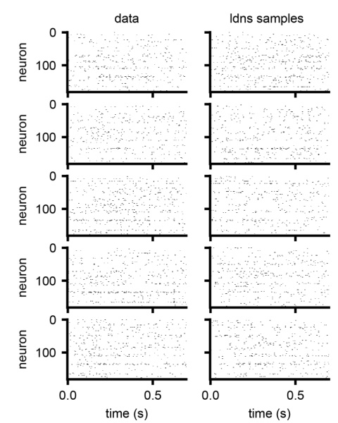
This figure visually compares spiking data generated by the LDNS model with real spiking data from the dataset. It shows five example trials, each with the real data on the left and the corresponding LDNS-generated samples on the right. This comparison helps to assess the quality and realism of the model’s output, showing how well the generated data matches the patterns and characteristics found in the real data.
This figure demonstrates the ability of LDNS to generate realistic neural spiking data for a monkey performing reach tasks in different mazes. It shows that LDNS accurately captures various aspects of the data, including population spike counts, pairwise correlations, and single-neuron inter-spike interval statistics, both with and without incorporating single-neuron dynamics using spike history.

This figure demonstrates the ability of LDNS to generate realistic synthetic spiking data with underlying chaotic dynamics. It shows that LDNS accurately recovers latent structure, firing rates, and spiking statistics from synthetic data generated by a Lorenz system. The figure compares the generated data to the original data across several metrics, showing a good match for both population-level and single-neuron properties.

This figure provides a visual comparison of spiking data generated by LDNS and several baseline methods (LFADS, LFADS with spike history, TNDM, and pi-VAE) against real neural spiking data. It shows raster plots for each method and the real data, allowing for a direct visual comparison of the spike patterns generated. This allows for a qualitative assessment of the various methods’ ability to replicate the temporal structure and characteristics of real neural data.
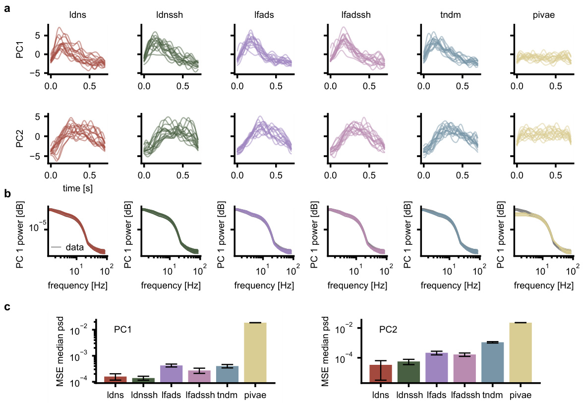
This figure compares the performance of LDNS and other models in capturing the temporal dynamics of neural data. Panel (a) shows the first two principal components of smoothed spike data from different models and real data. Panel (b) displays the power spectral density for the first principal component, highlighting differences in frequency representation among models. Panel (c) quantifies these differences using the mean squared error of the median power spectral density. The results show that LDNS and LDNSsh (with spike history) accurately capture the temporal dynamics of the data better than alternative models.
This figure demonstrates the ability of LDNS to generate realistic spiking data from a synthetic dataset based on the Lorenz attractor. It shows that LDNS accurately recovers latent structure, firing rates, and spiking statistics at both the population and single-neuron levels, even when generating data that is much longer than the training data.

This figure demonstrates the conditional generation capabilities of LDNS. Panel (a) shows the experimental setup for closed-loop assessment. Panels (b-d) show that LDNS can generate realistic neural activity when conditioned on reach direction or velocity. Panels (e-g) illustrate that the latent space learned by LDNS captures relevant information about reach kinematics. The smooth temporal variation of latents conditional on various trajectories and their clear clustering according to reach directions show the capability of LDNS in inferring meaningful representations of behavior.
More on tables
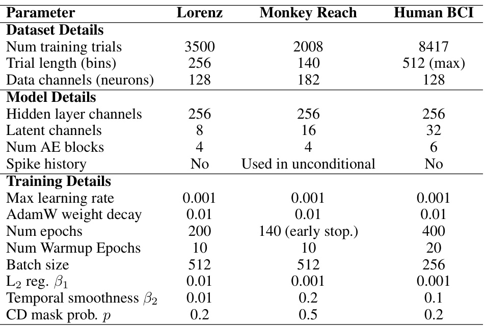
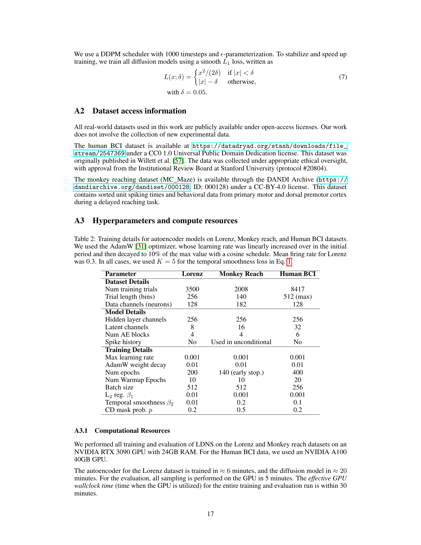
This table shows the hyperparameters used for training the autoencoder models for three different datasets: Lorenz, Monkey Reach, and Human BCI. The AdamW optimizer was used with a linearly increasing learning rate that decayed to 10% of its maximum value using a cosine schedule. For the Lorenz dataset, the mean firing rate was 0.3. In all cases, the temporal smoothness loss (Eq. 1) used K=5.
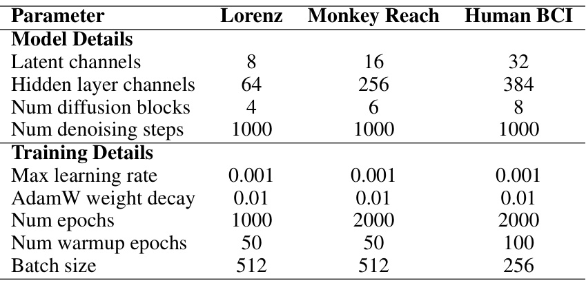
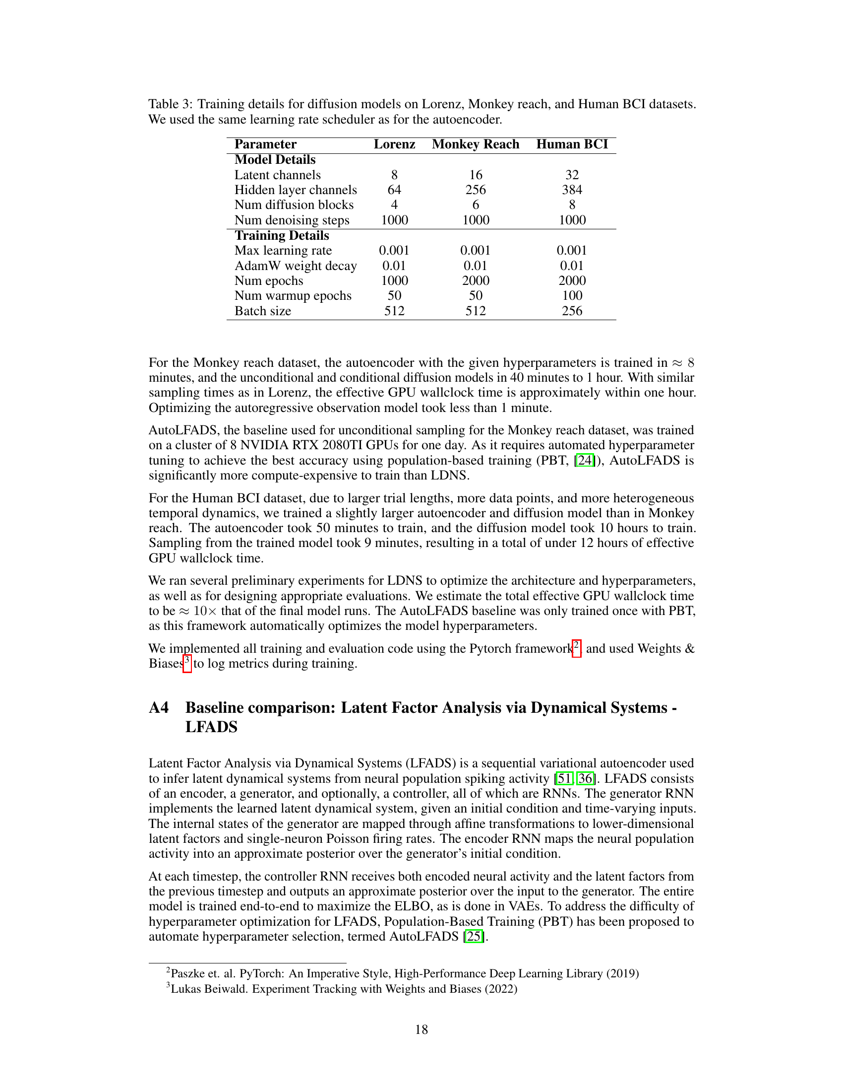
This table shows the hyperparameters used for training the diffusion models in the LDNS framework. It provides details on the model architecture (number of latent channels, hidden layer channels, diffusion blocks, and denoising steps) and the training process (maximum learning rate, AdamW weight decay, number of epochs, warmup epochs, and batch size). The hyperparameters are specific to each dataset: Lorenz, Monkey Reach, and Human BCI.

This table presents the quantitative comparison of different models’ performance on the monkey reach task dataset. The models compared are AutoLFADS, LDNS, AutoLFADSsh (AutoLFADS with spike history), and LDNSsh (LDNS with spike history). The metrics used for comparison are DKL (Kullback-Leibler divergence) for population spike count histogram, RMSE (root mean squared error) for pairwise correlations, RMSE for mean inter-spike intervals (isi), and RMSE for standard deviation of isi. The table shows that LDNSsh achieves the best performance across all the metrics.
Full paper#
